


15.5.1. Source Distribution Equations
The actual spectra of radio sources are normally approximated by power
laws so that the spectral luminosity function at all frequencies
 is determined by the
spectral luminosity function at any one frequency
0 from
is determined by the
spectral luminosity function at any one frequency
0 from
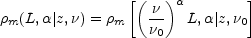 |
(15.17) |
for a measured between any two frequencies. Models based on this
approximation generally work well at
= 408 MHz and higher
frequencies, but they overestimate the 178-MHz source count significantly
(Peacock and Gull 1981,
Condon 1984b).
Both 178-MHz flux-density scale errors and genuine spectral curvature
caused by synchrotron self-absorption may contribute to this discrepancy.
The total number of sources with luminosities L to L +
dL spectral indices
 to
+
d, at frequency
, and lying in the spherical
shell with comoving volume dV at redshift z is
to
+
d, at frequency
, and lying in the spherical
shell with comoving volume dV at redshift z is
 |
(15.18) |
The number of sources in this shell equals the total number
 (S,
, z |
)
dS d dz of
sources with flux densities S to S + dS spectral
indices
to +
d, and redshifts
z to z + dz found in a survey of the whole sky
(4
(S,
, z |
)
dS d dz of
sources with flux densities S to S + dS spectral
indices
to +
d, and redshifts
z to z + dz found in a survey of the whole sky
(4 sr) at frequency
. Weighting by
S5/2 and eliminating both dV and dL /
dS yields
sr) at frequency
. Weighting by
S5/2 and eliminating both dV and dL /
dS yields
 |
(15.19) |
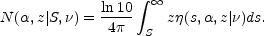
Integrating over redshift and dividing by
4 gives the weighted
(spectral) source count S5/2 n(S,
|
), where
n(S, |
) dS
d is the number of
sources per steradian with
flux densities S to S + dS and spectral indices
to
+
d found at
frequency :
 |
(15.20) |
The distribution equations (15.19) and (15.20) can be integrated
numerically to give the observables described in
Section 15.4. Using the
weighted luminosity function
 to calculate
the weighted source count directly minimizes the
interpolation errors that can be significant in numerical integrations
of the more rapidly varying luminosity function
to calculate
the weighted source count directly minimizes the
interpolation errors that can be significant in numerical integrations
of the more rapidly varying luminosity function
 m (cf.
Danese et al. 1983,
Peacock 1985)
to obtain the unweighted source count.
m (cf.
Danese et al. 1983,
Peacock 1985)
to obtain the unweighted source count.
The weighted differential source count S5/2
n(S |
) at frequency
(Section 15.4.2) is
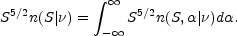 |
(15.21) |
The (unnormalized) spectral-index distribution
N( | S,
)
(Section 15.4.3) is obtained
by integrating the differential spectral count:
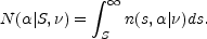 |
(15.22) |
The redshift/spectral-index diagram
(Section 15.4.4) shows the values of
N(, z |
S, ) given by
 |
(15.23) |
The (unnormalized) integral redshift distribution
N(z| S, )
(Section 15.4.5) is found by integrating over
:
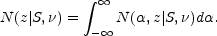 |
(15.24) |
Most radio sources in any flux-limited sample have flux densities only
slightly higher than the flux-density limit, so redshift and luminosity
are strongly correlated. Thus the integral luminosity distribution
N(L| S, )
can be used instead of the integral redshift distribution
N(z| S,
). Let
n(L, S,
|
) d[log(L)]dS
d, be the differential
number of sources per steradian with luminosities log(L) to
log(L) + d[log(L)], flux
densities S to S + dS and spectral indices
to
+
d at frequency
. Then,
4n(L, S,
|
) d[log(L)] =
(S,
, z |
) dz and
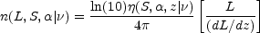 |
(15.25) |
where
 |
(15.26) |
and
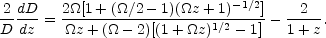 |
(15.27) |
Integrating Equation (15.25) over flux density and spectral index yields the (unnormalized) integral luminosity distribution
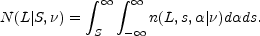 |
(15.28) |