


We now move from the domain of the weak-field limit to solutions of
the full nonlinear Einstein's equations. With the possible exception
of Minkowski space, by far the most important such solution is that
discovered by Schwarzschild, which describes spherically symmetric
vacuum spacetimes. Since we are in vacuum, Einstein's equations
become
R![]()
![]() = 0. Of course, if we have a proposed
solution to
a set of differential equations such as this, it would suffice to
plug in the proposed solution in order to verify it; we would like
to do better, however. In fact, we will sketch a proof of Birkhoff's
theorem, which states that the Schwarzschild solution is the unique
spherically symmetric solution to Einstein's equations in vacuum.
The procedure will be to first present some
non-rigorous arguments that any spherically symmetric metric (whether
or not it solves Einstein's equations) must take on a certain form,
and then work from there to more carefully derive the actual solution
in such a case.
= 0. Of course, if we have a proposed
solution to
a set of differential equations such as this, it would suffice to
plug in the proposed solution in order to verify it; we would like
to do better, however. In fact, we will sketch a proof of Birkhoff's
theorem, which states that the Schwarzschild solution is the unique
spherically symmetric solution to Einstein's equations in vacuum.
The procedure will be to first present some
non-rigorous arguments that any spherically symmetric metric (whether
or not it solves Einstein's equations) must take on a certain form,
and then work from there to more carefully derive the actual solution
in such a case.
"Spherically symmetric" means "having the same symmetries as a sphere." (In this section the word "sphere" means S2, not spheres of higher dimension.) Since the object of interest to us is the metric on a differentiable manifold, we are concerned with those metrics that have such symmetries. We know how to characterize symmetries of the metric - they are given by the existence of Killing vectors. Furthermore, we know what the Killing vectors of S2 are, and that there are three of them. Therefore, a spherically symmetric manifold is one that has three Killing vector fields which are just like those on S2. By "just like" we mean that the commutator of the Killing vectors is the same in either case - in fancier language, that the algebra generated by the vectors is the same. Something that we didn't show, but is true, is that we can choose our three Killing vectors on S2 to be (V(1), V(2), V(3)), such that
| (7.1) |
The commutation relations are exactly those of SO(3), the group of rotations in three dimensions. This is no coincidence, of course, but we won't pursue this here. All we need is that a spherically symmetric manifold is one which possesses three Killing vector fields with the above commutation relations.
Back in section three we mentioned Frobenius's Theorem, which states that if you have a set of commuting vector fields then there exists a set of coordinate functions such that the vector fields are the partial derivatives with respect to these functions. In fact the theorem does not stop there, but goes on to say that if we have some vector fields which do not commute, but whose commutator closes - the commutator of any two fields in the set is a linear combination of other fields in the set - then the integral curves of these vector fields "fit together" to describe submanifolds of the manifold on which they are all defined. The dimensionality of the submanifold may be smaller than the number of vectors, or it could be equal, but obviously not larger. Vector fields which obey (7.1) will of course form 2-spheres. Since the vector fields stretch throughout the space, every point will be on exactly one of these spheres. (Actually, it's almost every point - we will show below how it can fail to be absolutely every point.) Thus, we say that a spherically symmetric manifold can be foliated into spheres.
Let's consider some examples to bring this down to earth. The simplest
example is flat three-dimensional Euclidean space. If we pick an origin,
then ![]() is clearly spherically symmetric with respect to
rotations around this origin.
Under such rotations (i.e., under the
flow of the Killing vector fields) points move into each other, but
each point stays on an S2 at a fixed distance from the
origin.
is clearly spherically symmetric with respect to
rotations around this origin.
Under such rotations (i.e., under the
flow of the Killing vector fields) points move into each other, but
each point stays on an S2 at a fixed distance from the
origin.

|
It is these spheres which foliate ![]() .
Of course, they don't really foliate all of the space, since
the origin itself just stays put under rotations - it doesn't move
around on some two-sphere. But it should be clear that almost all of
the space is properly foliated, and this will turn out to be enough for
us.
.
Of course, they don't really foliate all of the space, since
the origin itself just stays put under rotations - it doesn't move
around on some two-sphere. But it should be clear that almost all of
the space is properly foliated, and this will turn out to be enough for
us.
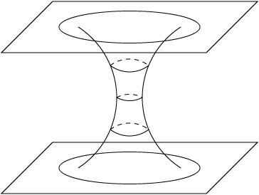
We can also have spherical symmetry without an "origin" to rotate
things around. An example is provided by a "wormhole", with topology
![]() × S2. If we suppress a
dimension and draw our two-spheres
as circles, such a space might look like this:
× S2. If we suppress a
dimension and draw our two-spheres
as circles, such a space might look like this:
|
In this case the entire manifold can be foliated by two-spheres.
This foliated structure suggests that we put coordinates on our manifold in a way which is adapted to the foliation. By this we mean that, if we have an n-dimensional manifold foliated by m-dimensional submanifolds, we can use a set of m coordinate functions ui on the submanifolds and a set of n - m coordinate functions vI to tell us which submanifold we are on. (So i runs from 1 to m, while I runs from 1 to n - m.) Then the collection of v's and u's coordinatize the entire space. If the submanifolds are maximally symmetric spaces (as two-spheres are), then there is the following powerful theorem: it is always possible to choose the u-coordinates such that the metric on the entire manifold is of the form

| (7.2) |
Here ![]() (u) is the metric on the submanifold.
This theorem is saying two things at once: that there are no cross
terms
dvIduj, and that both
gIJ(v) and f (v) are functions
of the vI alone, independent of the
ui. Proving the theorem is
a mess, but you are encouraged to look in chapter 13 of Weinberg.
Nevertheless, it is a perfectly sensible result. Roughly speaking,
if gIJ or f depended on the ui then the metric would change
as we moved in a single submanifold, which violates the assumption of
symmetry. The unwanted cross terms, meanwhile, can be eliminated by
making sure that the tangent vectors
(u) is the metric on the submanifold.
This theorem is saying two things at once: that there are no cross
terms
dvIduj, and that both
gIJ(v) and f (v) are functions
of the vI alone, independent of the
ui. Proving the theorem is
a mess, but you are encouraged to look in chapter 13 of Weinberg.
Nevertheless, it is a perfectly sensible result. Roughly speaking,
if gIJ or f depended on the ui then the metric would change
as we moved in a single submanifold, which violates the assumption of
symmetry. The unwanted cross terms, meanwhile, can be eliminated by
making sure that the tangent vectors
![]() /
/![]() vI are
orthogonal to the submanifolds - in other words, that
we line up our submanifolds in the same way throughout the space.
vI are
orthogonal to the submanifolds - in other words, that
we line up our submanifolds in the same way throughout the space.
We are now through with handwaving, and can commence some honest
calculation.
For the case at hand, our submanifolds are two-spheres, on which we
typically choose coordinates
(![]() ,
,![]() ) in which the metric takes
the form
) in which the metric takes
the form
| (7.3) |
Since we are interested in a four-dimensional spacetime, we need two more coordinates, which we can call a and b. The theorem (7.2) is then telling us that the metric on a spherically symmetric spacetime can be put in the form

| (7.4) |
Here r(a, b) is some as-yet-undetermined function, to which we have merely given a suggestive label. There is nothing to stop us, however, from changing coordinates from (a, b) to (a, r), by inverting r(a, b). (The one thing that could possibly stop us would be if r were a function of a alone; in this case we could just as easily switch to (b, r), so we will not consider this situation separately.) The metric is then

| (7.5) |
Our next step is to find a function t(a, r) such that, in the (t, r) coordinate system, there are no cross terms dtdr + drdt in the metric. Notice that
| (7.6) |
so
| (7.7) |
We would like to replace the first three terms in the metric (7.5) by

| (7.8) |
for some functions m and n. This is equivalent to the requirements
| (7.9) |
| (7.10) |
and
| (7.11) |
We therefore have three equations for the three unknowns t(a, r), m(a, r), and n(a, r), just enough to determine them precisely (up to initial conditions for t). (Of course, they are "determined" in terms of the unknown functions gaa, gar, and grr, so in this sense they are still undetermined.) We can therefore put our metric in the form
| (7.12) |
To this point the only difference between the two coordinates t and
r is that we have chosen r to be the one which multiplies the
metric for the two-sphere. This choice was motivated by what we know
about the metric for flat Minkowski space, which can be written
ds2 = - dt2 + dr2
+ r2d![]() . We know that the spacetime
under consideration is Lorentzian, so either m or n will
have to be negative. Let us choose m, the coefficient of
dt2, to be
negative. This is not a choice we are simply allowed to make, and in
fact we will see later that it can go wrong, but we will assume it for
now. The assumption is not completely unreasonable, since we know that
Minkowski space is itself spherically symmetric, and will therefore be
described by (7.12). With this choice we can trade in the functions
m and n for new functions
. We know that the spacetime
under consideration is Lorentzian, so either m or n will
have to be negative. Let us choose m, the coefficient of
dt2, to be
negative. This is not a choice we are simply allowed to make, and in
fact we will see later that it can go wrong, but we will assume it for
now. The assumption is not completely unreasonable, since we know that
Minkowski space is itself spherically symmetric, and will therefore be
described by (7.12). With this choice we can trade in the functions
m and n for new functions ![]() and
and ![]() , such that
, such that

| (7.13) |
This is the best we can do for a general metric in a spherically
symmetric spacetime. The next step is to actually solve Einstein's
equations, which will allow us to determine explicitly the functions
![]() (t, r) and
(t, r) and
![]() (t, r). It is unfortunately necessary to
compute the Christoffel symbols for (7.13), from which we can get
the curvature tensor and thus the Ricci tensor. If we use labels
(0, 1, 2, 3) for
(t, r,
(t, r). It is unfortunately necessary to
compute the Christoffel symbols for (7.13), from which we can get
the curvature tensor and thus the Ricci tensor. If we use labels
(0, 1, 2, 3) for
(t, r,![]() ,
,![]() ) in the usual way, the Christoffel
symbols are given by
) in the usual way, the Christoffel
symbols are given by
| (7.14) |
(Anything not written down explicitly is meant to be zero, or related to what is written by symmetries.) From these we get the following nonvanishing components of the Riemann tensor:
| (7.15) |
Taking the contraction as usual yields the Ricci tensor:
| (7.16) |
Our job is to set R![]()
![]() = 0. From R01 = 0 we
get
= 0. From R01 = 0 we
get

| (7.17) |
If we consider taking the time derivative of R22 = 0
and using
![]()
![]() = 0, we get
= 0, we get

| (7.18) |
We can therefore write
| (7.19) |
The first term in the metric (7.13) is therefore
- e2f(r)e2g(t)dt2.
But we could always simply redefine our time coordinate by
replacing
dt ![]() e-g(t)dt; in other
words, we are free
to choose t such that g(t) = 0, whence
e-g(t)dt; in other
words, we are free
to choose t such that g(t) = 0, whence
![]() (t, r) = f (r). We therefore
have
(t, r) = f (r). We therefore
have

| (7.20) |
All of the metric components are independent of the coordinate t. We have therefore proven a crucial result: any spherically symmetric vacuum metric possesses a timelike Killing vector.
This property is so interesting that it gets its own name: a metric
which possesses a timelike Killing vector is called stationary.
There is also a more restrictive property: a metric is called
static if it possesses a timelike Killing vector which is
orthogonal to a family of hypersurfaces. (A hypersurface in an
n-dimensional manifold is simply an (n - 1)-dimensional
submanifold.) The metric (7.20) is not
only stationary, but also static; the Killing vector field
![]() is
orthogonal to the surfaces t = const (since there are no
cross terms such as
dtdr and so on). Roughly speaking, a static metric is
one in which nothing is moving, while a stationary metric allows things
to move but only in a symmetric way. For example, the static spherically
symmetric metric (7.20) will describe non-rotating stars or black holes,
while rotating systems (which keep rotating in the same way at all times)
will be described by stationary metrics. It's hard to remember which
word goes with which concept, but the distinction between the two
concepts should be understandable.
is
orthogonal to the surfaces t = const (since there are no
cross terms such as
dtdr and so on). Roughly speaking, a static metric is
one in which nothing is moving, while a stationary metric allows things
to move but only in a symmetric way. For example, the static spherically
symmetric metric (7.20) will describe non-rotating stars or black holes,
while rotating systems (which keep rotating in the same way at all times)
will be described by stationary metrics. It's hard to remember which
word goes with which concept, but the distinction between the two
concepts should be understandable.
Let's keep going with finding the solution. Since both R00 and R11 vanish, we can write
| (7.21) |
which implies
![]() = -
= - ![]() + constant. Once again, we can
get rid of the constant by scaling our coordinates, so we have
+ constant. Once again, we can
get rid of the constant by scaling our coordinates, so we have

| (7.22) |
Next let us turn to R22 = 0, which now reads
| (7.23) |
This is completely equivalent to

| (7.24) |
We can solve this to obtain

| (7.25) |
where ![]() is some undetermined constant. With (7.22) and (7.25),
our metric becomes
is some undetermined constant. With (7.22) and (7.25),
our metric becomes
| (7.26) |
We now have no freedom left except for the single constant ![]() , so
this form better solve the remaining equations R00 = 0 and
R11 = 0; it is straightforward to check that it does,
for any value of
, so
this form better solve the remaining equations R00 = 0 and
R11 = 0; it is straightforward to check that it does,
for any value of ![]() .
.
The only thing left to do is to interpret the constant ![]() in
terms of some physical parameter. The most important use of a
spherically symmetric vacuum solution is to represent the spacetime
outside a star or planet or whatnot. In that case we would expect
to recover the weak field limit as
r
in
terms of some physical parameter. The most important use of a
spherically symmetric vacuum solution is to represent the spacetime
outside a star or planet or whatnot. In that case we would expect
to recover the weak field limit as
r ![]()
![]() . In this
limit, (7.26) implies
. In this
limit, (7.26) implies
| (7.27) |
The weak field limit, on the other hand, has
| (7.28) |
with the potential
![]() = - GM/r. Therefore the metrics do agree in
this limit, if we set
= - GM/r. Therefore the metrics do agree in
this limit, if we set
![]() = - 2GM.
= - 2GM.
Our final result is the celebrated Schwarzschild metric,
| (7.29) |
This is true for any spherically symmetric vacuum solution to
Einstein's equations; M functions as a parameter, which we happen
to know can be interpreted as the conventional Newtonian mass that we
would measure by studying orbits at large distances from the
gravitating source. Note that as
M ![]() 0 we recover
Minkowski space, which is to be expected. Note also that the metric
becomes progressively Minkowskian as we go to
r
0 we recover
Minkowski space, which is to be expected. Note also that the metric
becomes progressively Minkowskian as we go to
r ![]()
![]() ;
this property is known as asymptotic flatness.
;
this property is known as asymptotic flatness.
The fact that the Schwarzschild metric is not just a good solution, but is the unique spherically symmetric vacuum solution, is known as Birkhoff's theorem. It is interesting to note that the result is a static metric. We did not say anything about the source except that it be spherically symmetric. Specifically, we did not demand that the source itself be static; it could be a collapsing star, as long as the collapse were symmetric. Therefore a process such as a supernova explosion, which is basically spherical, would be expected to generate very little gravitational radiation (in comparison to the amount of energy released through other channels). This is the same result we would have obtained in electromagnetism, where the electromagnetic fields around a spherical charge distribution do not depend on the radial distribution of the charges.
Before exploring the behavior of test particles in the Schwarzschild
geometry, we should say something about singularities. From the form
of (7.29), the metric coefficients become infinite at r = 0 and
r = 2GM - an apparent sign that something is going
wrong. The metric coefficients, of course, are
coordinate-dependent quantities, and as such we should not make too
much of their values; it is certainly possible to have a "coordinate
singularity" which results from a breakdown of a specific coordinate
system rather than the underlying manifold. An example occurs at
the origin of polar coordinates in the plane, where the metric
ds2 = dr2 +
r2d![]() becomes degenerate and the component
g
becomes degenerate and the component
g![]()
![]() = r-2 of the
inverse metric blows up, even
though that point of the manifold is no different from any other.
= r-2 of the
inverse metric blows up, even
though that point of the manifold is no different from any other.
What kind of coordinate-independent signal should
we look for as a warning that something about the geometry is out of
control? This turns out to be a difficult question to answer, and
entire books have been written about the nature of singularities in
general relativity. We won't go into this issue in detail, but
rather turn to one simple criterion for when something has gone wrong -
when the curvature becomes infinite. The curvature is measured by
the Riemann tensor, and it is hard to say when a tensor becomes infinite,
since its components are coordinate-dependent. But from the curvature
we can construct various scalar quantities, and since scalars are
coordinate-independent it will be meaningful to say that they become
infinite. This simplest such scalar is the Ricci scalar
R = g![]()
![]() R
R![]()
![]() ,
but we can also construct higher-order scalars such as
R
,
but we can also construct higher-order scalars such as
R![]()
![]() R
R![]()
![]() ,
R
,
R![]()
![]()
![]()
![]() R
R![]()
![]()
![]()
![]() ,
R
,
R![]()
![]()
![]()
![]() R
R![]()
![]()
![]()
![]() R
R![]()
![]()
![]()
![]() , and so on. If any
of these scalars (not necessarily all of them) go to infinity as we
approach some point, we will regard that point as a singularity of the
curvature. We should also check that the point is not "infinitely
far away"; that is, that it can be reached by travelling a finite
distance along a curve.
, and so on. If any
of these scalars (not necessarily all of them) go to infinity as we
approach some point, we will regard that point as a singularity of the
curvature. We should also check that the point is not "infinitely
far away"; that is, that it can be reached by travelling a finite
distance along a curve.
We therefore have a sufficient condition for a point to be considered a singularity. It is not a necessary condition, however, and it is generally harder to show that a given point is nonsingular; for our purposes we will simply test to see if geodesics are well-behaved at the point in question, and if so then we will consider the point nonsingular. In the case of the Schwarzschild metric (7.29), direct calculation reveals that
| (7.30) |
This is enough to convince us that r = 0 represents an honest singularity. At the other trouble spot, r = 2GM, you could check and see that none of the curvature invariants blows up. We therefore begin to think that it is actually not singular, and we have simply chosen a bad coordinate system. The best thing to do is to transform to more appropriate coordinates if possible. We will soon see that in this case it is in fact possible, and the surface r = 2GM is very well-behaved (although interesting) in the Schwarzschild metric.
Having worried a little about singularities, we should point out that
the behavior of Schwarzschild at r ![]() 2GM is of little day-to-day
consequence. The solution we derived is valid only in vacuum, and
we expect it to hold outside a spherical body such as a star. However,
in the case of the Sun we are dealing with a body which extends to a
radius of
2GM is of little day-to-day
consequence. The solution we derived is valid only in vacuum, and
we expect it to hold outside a spherical body such as a star. However,
in the case of the Sun we are dealing with a body which extends to a
radius of
| (7.31) |
Thus, r = 2GM![]() is far inside the solar interior,
where we do not
expect the Schwarzschild metric to imply. In fact, realistic stellar
interior solutions are of the form
is far inside the solar interior,
where we do not
expect the Schwarzschild metric to imply. In fact, realistic stellar
interior solutions are of the form
| (7.32) |
See Schutz for details. Here m(r) is a function of r which goes to zero faster than r itself, so there are no singularities to deal with at all. Nevertheless, there are objects for which the full Schwarzschild metric is required - black holes - and therefore we will let our imaginations roam far outside the solar system in this section.
The first step we will take to understand this metric more fully is to consider the behavior of geodesics. We need the nonzero Christoffel symbols for Schwarzschild:
| (7.33) |
The geodesic equation therefore turns into the following four
equations, where ![]() is an affine parameter:
is an affine parameter:
| (7.34) |
| (7.35) |
| (7.36) |
and
| (7.37) |
There does not seem to be much hope for simply solving this set of
coupled equations by inspection. Fortunately our task is greatly
simplified by the high degree of symmetry of the Schwarzschild metric.
We know that there are four Killing vectors: three for the spherical
symmetry, and one for time translations. Each of these will lead to
a constant of the motion for a free particle; if K![]() is a Killing
vector, we know that
is a Killing
vector, we know that
| (7.38) |
In addition, there is another constant of the motion that we always have for geodesics; metric compatibility implies that along the path the quantity
| (7.39) |
is constant.
Of course, for a massive particle we typically choose
![]() =
= ![]() ,
and this relation simply becomes
,
and this relation simply becomes
![]() = - g
= - g![]()
![]() U
U![]() U
U![]() = + 1. For
a massless particle we always have
= + 1. For
a massless particle we always have
![]() = 0. We will also be
concerned with spacelike geodesics (even though they do not correspond
to paths of particles), for which we will choose
= 0. We will also be
concerned with spacelike geodesics (even though they do not correspond
to paths of particles), for which we will choose
![]() = - 1.
= - 1.
Rather than immediately writing out explicit expressions for the four conserved quantities associated with Killing vectors, let's think about what they are telling us. Notice that the symmetries they represent are also present in flat spacetime, where the conserved quantities they lead to are very familiar. Invariance under time translations leads to conservation of energy, while invariance under spatial rotations leads to conservation of the three components of angular momentum. Essentially the same applies to the Schwarzschild metric. We can think of the angular momentum as a three-vector with a magnitude (one component) and direction (two components). Conservation of the direction of angular momentum means that the particle will move in a plane. We can choose this to be the equatorial plane of our coordinate system; if the particle is not in this plane, we can rotate coordinates until it is. Thus, the two Killing vectors which lead to conservation of the direction of angular momentum imply

| (7.40) |
The two remaining Killing vectors correspond to energy and the
magnitude of angular momentum. The energy arises from the timelike
Killing vector K = ![]() , or
, or
| (7.41) |
The Killing vector whose conserved quantity is the magnitude of the
angular momentum is L = ![]() , or
, or
| (7.42) |
Since (7.40) implies that
sin![]() = 1 along the geodesics of
interest to us, the two conserved quantities are
= 1 along the geodesics of
interest to us, the two conserved quantities are
| (7.43) |
and

| (7.44) |
For massless particles these can be thought of as the energy and angular momentum; for massive particles they are the energy and angular momentum per unit mass of the particle. Note that the constancy of (7.44) is the GR equivalent of Kepler's second law (equal areas are swept out in equal times).
Together these conserved quantities provide a convenient way to
understand the orbits of particles in the Schwarzschild geometry.
Let us expand the expression (7.39) for ![]() to obtain
to obtain
| (7.45) |
If we multiply this by (1 - 2GM/r) and use our expressions for E and L, we obtain
| (7.46) |
This is certainly progress, since we have taken a messy system of
coupled equations and obtained a single equation for
r(![]() ).
It looks even nicer if we rewrite it as
).
It looks even nicer if we rewrite it as
| (7.47) |
where
| (7.48) |
In (7.47) we have precisely the equation for a classical particle of unit
mass and "energy"
![]() E2 moving in a one-dimensional
potential
given by V(r). (The true energy per unit mass is E,
but the
effective potential for the coordinate r responds to
E2 moving in a one-dimensional
potential
given by V(r). (The true energy per unit mass is E,
but the
effective potential for the coordinate r responds to
![]() E2.)
E2.)
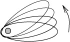
Of course, our physical situation is quite different from a classical particle moving in one dimension. The trajectories under consideration are orbits around a star or other object:
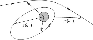
|
The quantities of interest to us are not only
r(![]() ),
but also t(
),
but also t(![]() ) and
) and
![]() (
(![]() ). Nevertheless, we can go a
long way toward understanding all of the orbits by understanding their
radial behavior, and it is a great help to reduce this behavior to a
problem we know how to solve.
). Nevertheless, we can go a
long way toward understanding all of the orbits by understanding their
radial behavior, and it is a great help to reduce this behavior to a
problem we know how to solve.
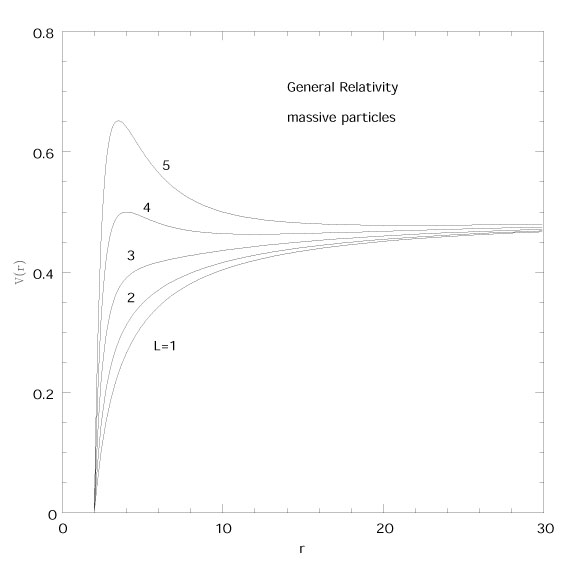
A similar analysis of orbits in Newtonian gravity would have produced a similar result; the general equation (7.47) would have been the same, but the effective potential (7.48) would not have had the last term. (Note that this equation is not a power series in 1/r, it is exact.) In the potential (7.48) the first term is just a constant, the second term corresponds exactly to the Newtonian gravitational potential, and the third term is a contribution from angular momentum which takes the same form in Newtonian gravity and general relativity. The last term, the GR contribution, will turn out to make a great deal of difference, especially at small r.
Let us examine the kinds of possible orbits, as illustrated in the
figures. There are different curves V(r) for different values
of L; for any one of these curves, the behavior of the orbit can be
judged by comparing the
![]() E2 to V(r). The
general behavior of
the particle will be to move in the potential until it reaches a
"turning point" where
V(r) =
E2 to V(r). The
general behavior of
the particle will be to move in the potential until it reaches a
"turning point" where
V(r) = ![]() E2, where it will begin moving
in the other direction. Sometimes there may be no turning point to hit,
in which case the particle just keeps going. In other cases the
particle may simply move in a circular orbit at radius
rc = const; this
can happen if the potential is flat, dV/dr =
0. Differentiating
(7.48), we find that the circular orbits occur when
E2, where it will begin moving
in the other direction. Sometimes there may be no turning point to hit,
in which case the particle just keeps going. In other cases the
particle may simply move in a circular orbit at radius
rc = const; this
can happen if the potential is flat, dV/dr =
0. Differentiating
(7.48), we find that the circular orbits occur when
| (7.49) |
where ![]() = 0 in Newtonian gravity and
= 0 in Newtonian gravity and ![]() = 1 in general
relativity. Circular orbits will be stable if they correspond to
a minimum of the potential, and unstable if they correspond to a
maximum. Bound orbits which are not circular will oscillate
around the radius of the stable circular orbit.
= 1 in general
relativity. Circular orbits will be stable if they correspond to
a minimum of the potential, and unstable if they correspond to a
maximum. Bound orbits which are not circular will oscillate
around the radius of the stable circular orbit.
|
|
Turning to Newtonian gravity, we find that circular orbits appear at

| (7.50) |
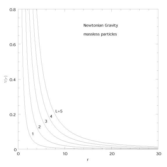
For massless particles
![]() = 0, and there are no circular orbits;
this is consistent with the figure, which illustrates that there are no
bound orbits of any sort. Although it is somewhat obscured in this
coordinate system, massless particles actually move in a straight
line, since the Newtonian gravitational force on a massless particle is
zero. (Of course the standing of massless particles in Newtonian theory
is somewhat problematic, but we will ignore that for now.) In terms of
the effective potential, a photon with a given energy E will come in
from r =
= 0, and there are no circular orbits;
this is consistent with the figure, which illustrates that there are no
bound orbits of any sort. Although it is somewhat obscured in this
coordinate system, massless particles actually move in a straight
line, since the Newtonian gravitational force on a massless particle is
zero. (Of course the standing of massless particles in Newtonian theory
is somewhat problematic, but we will ignore that for now.) In terms of
the effective potential, a photon with a given energy E will come in
from r = ![]() and gradually "slow down" (actually
dr/d
and gradually "slow down" (actually
dr/d![]() will decrease, but the speed of light isn't changing) until it reaches
the turning point, when it will start moving away back to
r =
will decrease, but the speed of light isn't changing) until it reaches
the turning point, when it will start moving away back to
r = ![]() . The lower values of L, for which the photon
will come
closer before it starts moving away, are simply those trajectories which
are initially aimed closer to the gravitating body.
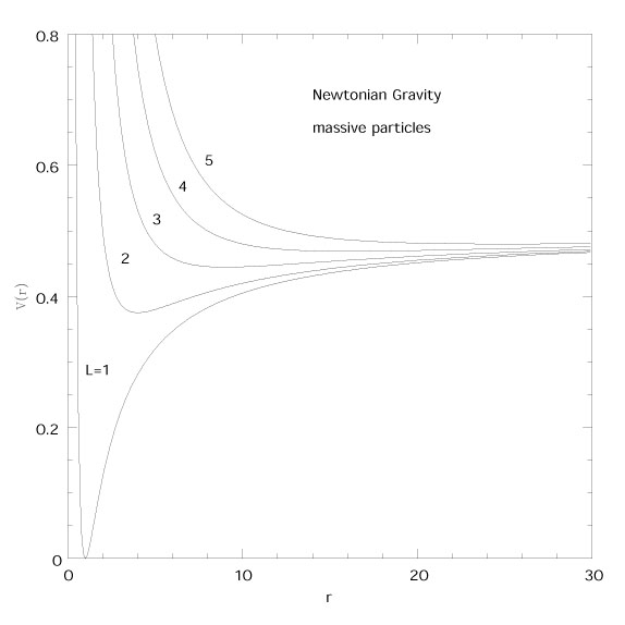
For massive particles there will be stable circular orbits at the
radius (7.50), as well as bound orbits which oscillate around this
radius. If the energy is greater than the asymptotic value E = 1,
the orbits will be unbound, describing a particle that approaches the
star and then recedes. We know that the orbits in Newton's theory are
conic sections - bound orbits are either circles or ellipses, while
unbound ones are either parabolas or hyperbolas - although we won't
show that here.
. The lower values of L, for which the photon
will come
closer before it starts moving away, are simply those trajectories which
are initially aimed closer to the gravitating body.
For massive particles there will be stable circular orbits at the
radius (7.50), as well as bound orbits which oscillate around this
radius. If the energy is greater than the asymptotic value E = 1,
the orbits will be unbound, describing a particle that approaches the
star and then recedes. We know that the orbits in Newton's theory are
conic sections - bound orbits are either circles or ellipses, while
unbound ones are either parabolas or hyperbolas - although we won't
show that here.
In general relativity the situation is different, but only for r
sufficiently small. Since the difference resides in the term
- GML2/r3, as
r ![]()
![]() the behaviors are identical in the two
theories. But as
r
the behaviors are identical in the two
theories. But as
r ![]() 0 the potential goes to -
0 the potential goes to - ![]() rather than +
rather than + ![]() as in the Newtonian case. At r = 2GM the
potential is always zero; inside this radius is the black hole, which
we will discuss more thoroughly later. For massless particles
there is always a barrier (except for L = 0, for which the potential
vanishes identically), but a sufficiently energetic photon will
nevertheless go over the barrier and be dragged inexorably down to
the center. (Note that "sufficiently energetic" means "in comparison
to its angular momentum" - in fact the frequency of the photon is
immaterial, only the direction in which it is pointing.) At the top
of the barrier there are unstable circular orbits.
For
as in the Newtonian case. At r = 2GM the
potential is always zero; inside this radius is the black hole, which
we will discuss more thoroughly later. For massless particles
there is always a barrier (except for L = 0, for which the potential
vanishes identically), but a sufficiently energetic photon will
nevertheless go over the barrier and be dragged inexorably down to
the center. (Note that "sufficiently energetic" means "in comparison
to its angular momentum" - in fact the frequency of the photon is
immaterial, only the direction in which it is pointing.) At the top
of the barrier there are unstable circular orbits.
For
![]() = 0,
= 0, ![]() = 1, we can easily solve (7.49) to obtain
= 1, we can easily solve (7.49) to obtain

| (7.51) |
This is borne out by the figure, which shows a maximum of
V(r) at
r = 3GM for every L. This means that a photon can
orbit forever in a circle at this radius, but any
perturbation will cause it to fly away either to r = 0 or
r = ![]() .
.
|

|
For massive particles there are once again different regimes depending on the angular momentum. The circular orbits are at
| (7.52) |
For large L there will be two circular orbits, one stable and one
unstable. In the
L ![]()
![]() limit their radii are given by
limit their radii are given by
| (7.53) |
In this limit the stable circular orbit becomes farther and farther away, while the unstable one approaches 3GM, behavior which parallels the massless case. As we decrease L the two circular orbits come closer together; they coincide when the discriminant in (7.52) vanishes, at

| (7.54) |
for which

| (7.55) |
and disappear entirely for smaller L. Thus 6GM is the
smallest possible radius of a stable circular orbit in the
Schwarzschild metric. There are also unbound orbits, which come in
from infinity and turn around, and bound but noncircular ones, which
oscillate around the stable circular radius. Note that such
orbits, which would describe exact conic sections in
Newtonian gravity, will not do so in GR, although we would have to
solve the equation for d![]() /dt to demonstrate it. Finally, there are
orbits which come in from infinity and continue all the way in to
r = 0; this can happen either if the energy is higher than the
barrier, or for
L <
/dt to demonstrate it. Finally, there are
orbits which come in from infinity and continue all the way in to
r = 0; this can happen either if the energy is higher than the
barrier, or for
L < ![]() GM, when the barrier goes away entirely.
GM, when the barrier goes away entirely.
We have therefore found that the Schwarzschild solution possesses stable circular orbits for r > 6GM and unstable circular orbits for 3GM < r < 6GM. It's important to remember that these are only the geodesics; there is nothing to stop an accelerating particle from dipping below r = 3GM and emerging, as long as it stays beyond r = 2GM.
Most experimental tests of general relativity involve the motion of test particles in the solar system, and hence geodesics of the Schwarzschild metric; this is therefore a good place to pause and consider these tests. Einstein suggested three tests: the deflection of light, the precession of perihelia, and gravitational redshift. The deflection of light is observable in the weak-field limit, and therefore is not really a good test of the exact form of the Schwarzschild geometry. Observations of this deflection have been performed during eclipses of the Sun, with results which agree with the GR prediction (although it's not an especially clean experiment). The precession of perihelia reflects the fact that noncircular orbits are not closed ellipses; to a good approximation they are ellipses which precess, describing a flower pattern.
|
Using our geodesic equations, we could solve for
d![]() /d
/d![]() as a power series in the eccentricity e of the
orbit, and from that obtain the apsidal frequency
as a power series in the eccentricity e of the
orbit, and from that obtain the apsidal frequency ![]() ,
defined as 2
,
defined as 2![]() divided by the time it takes for the ellipse to
precess once around.
For details you can look in Weinberg; the answer is
divided by the time it takes for the ellipse to
precess once around.
For details you can look in Weinberg; the answer is
| (7.56) |
where we have restored the c to make it easier to compare with observation. (It is a good exercise to derive this yourself to lowest nonvanishing order, in which case the e2 is missing.) Historically the precession of Mercury was the first test of GR. For Mercury the relevant numbers are
| (7.57) |
and of course
c = 3.00 × 1010 cm/sec. This gives
![]() = 2.35 × 10⁻¹⁴
sec-1. In other words, the major axis
of Mercury's orbit precesses at a rate of 42.9 arcsecs every 100
years. The observed value is 5601 arcsecs/100 yrs. However,
much of that is due to the precession of equinoxes in our geocentric
coordinate system; 5025 arcsecs/100 yrs, to be precise. The
gravitational perturbations of the other planets contribute an
additional 532 arcsecs/100 yrs, leaving 43 arcsecs/100 yrs
to be explained by GR, which it does quite well.
= 2.35 × 10⁻¹⁴
sec-1. In other words, the major axis
of Mercury's orbit precesses at a rate of 42.9 arcsecs every 100
years. The observed value is 5601 arcsecs/100 yrs. However,
much of that is due to the precession of equinoxes in our geocentric
coordinate system; 5025 arcsecs/100 yrs, to be precise. The
gravitational perturbations of the other planets contribute an
additional 532 arcsecs/100 yrs, leaving 43 arcsecs/100 yrs
to be explained by GR, which it does quite well.
The gravitational redshift, as we have seen, is another effect
which is present in the weak field limit, and in fact will be predicted
by any theory of gravity which obeys the Principle of Equivalence.
However, this only applies to small enough regions of spacetime; over
larger distances, the exact amount of redshift will depend on the
metric, and thus on the theory under question. It is therefore
worth computing the redshift in the Schwarzschild geometry. We
consider two observers who are not moving on geodesics, but are stuck
at fixed spatial coordinate values
(r1,![]() ,
,![]() ) and
(r2,
) and
(r2,![]() ,
,![]() ). According to (7.45), the proper time of
observer i will be related to the coordinate time t by
). According to (7.45), the proper time of
observer i will be related to the coordinate time t by
| (7.58) |
Suppose that the observer
![]() 1 emits a light pulse which travels
to the observer
1 emits a light pulse which travels
to the observer
![]() 2, such that
2, such that
![]() 1 measures the time
between two successive crests of the light wave to be
1 measures the time
between two successive crests of the light wave to be
![]()
![]() .
Each crest follows the same path to
.
Each crest follows the same path to
![]() 2, except that they
are separated by a coordinate time
2, except that they
are separated by a coordinate time
| (7.59) |
This separation in coordinate time does not change along the photon trajectories, but the second observer measures a time between successive crests given by
| (7.60) |
Since these intervals
![]()
![]() measure the proper time between
two crests of an electromagnetic wave, the observed frequencies will be
related by
measure the proper time between
two crests of an electromagnetic wave, the observed frequencies will be
related by
| (7.61) |
This is an exact result for the frequency shift; in the limit r >> 2GM we have
| (7.62) |
This tells us that the frequency goes down as ![]() increases, which
happens as we climb out of a gravitational field; thus, a redshift.
You can check that it agrees with our previous calculation based on
the equivalence principle.
increases, which
happens as we climb out of a gravitational field; thus, a redshift.
You can check that it agrees with our previous calculation based on
the equivalence principle.
Since Einstein's proposal of the three classic tests, further tests of GR have been proposed. The most famous is of course the binary pulsar, discussed in the previous section. Another is the gravitational time delay, discovered by (and observed by) Shapiro. This is just the fact that the time elapsed along two different trajectories between two events need not be the same. It has been measured by reflecting radar signals off of Venus and Mars, and once again is consistent with the GR prediction. One effect which has not yet been observed is the Lense-Thirring, or frame-dragging effect. There has been a long-term effort devoted to a proposed satellite, dubbed Gravity Probe B, which would involve extraordinarily precise gyroscopes whose precession could be measured and the contribution from GR sorted out. It has a ways to go before being launched, however, and the survival of such projects is always year-to-year.
We now know something about the behavior of geodesics outside the troublesome radius r = 2GM, which is the regime of interest for the solar system and most other astrophysical situations. We will next turn to the study of objects which are described by the Schwarzschild solution even at radii smaller than 2GM - black holes. (We'll use the term "black hole" for the moment, even though we haven't introduced a precise meaning for such an object.)
One way of understanding a geometry is to explore its causal structure,
as defined by the light cones. We therefore consider radial null curves,
those for which ![]() and
and ![]() are constant and ds2 = 0:
are constant and ds2 = 0:
| (7.63) |
from which we see that
| (7.64) |
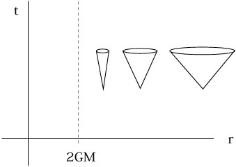
This of course measures the slope of the light cones on a spacetime diagram
of the t-r plane. For large r the slope is ±1,
as it would
be in flat space, while as we approach r = 2GM we get
dt/dr ![]() ±
±![]() , and the light cones "close up":
, and the light cones "close up":
|
Thus a light ray which approaches r = 2GM never seems to get there, at least in this coordinate system; instead it seems to asymptote to this radius.
As we will see, this is an illusion, and the light ray (or a massive particle) actually has no trouble reaching r = 2GM. But an observer far away would never be able to tell. If we stayed outside while an intrepid observational general relativist dove into the black hole, sending back signals all the time, we would simply see the signals reach us more and more slowly.
|
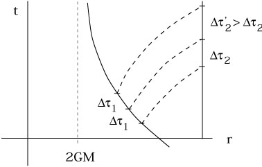
This should be clear from the pictures, and is confirmed
by our computation of
![]()
![]() /
/![]()
![]() when we discussed
the gravitational redshift (7.61). As infalling astronauts
approach r = 2GM, any fixed interval
when we discussed
the gravitational redshift (7.61). As infalling astronauts
approach r = 2GM, any fixed interval
![]()
![]() of their proper
time corresponds to a longer and longer interval
of their proper
time corresponds to a longer and longer interval
![]()
![]() from our point of view. This continues forever; we would never see
the astronaut cross r = 2GM, we would just see them move
more and
more slowly (and become redder and redder, almost as if they were
embarrassed to have done something as stupid as diving into a black hole).
from our point of view. This continues forever; we would never see
the astronaut cross r = 2GM, we would just see them move
more and
more slowly (and become redder and redder, almost as if they were
embarrassed to have done something as stupid as diving into a black hole).
The fact that we never see the infalling astronauts reach r = 2GM is a meaningful statement, but the fact that their trajectory in the t-r plane never reaches there is not. It is highly dependent on our coordinate system, and we would like to ask a more coordinate-independent question (such as, do the astronauts reach this radius in a finite amount of their proper time?). The best way to do this is to change coordinates to a system which is better behaved at r = 2GM. There does exist a set of such coordinates, which we now set out to find. There is no way to "derive" a coordinate transformation, of course, we just say what the new coordinates are and plug in the formulas. But we will develop these coordinates in several steps, in hopes of making the choices seem somewhat motivated.
The problem with our current coordinates is that
dt/dr ![]()
![]() along radial null geodesics which approach
r = 2GM; progress in the r direction becomes slower
and slower with
respect to the coordinate time t. We can try to fix this problem
by replacing t with a coordinate which "moves more slowly" along
null geodesics. First notice that we can explicitly solve the
condition (7.64) characterizing radial null curves to obtain
along radial null geodesics which approach
r = 2GM; progress in the r direction becomes slower
and slower with
respect to the coordinate time t. We can try to fix this problem
by replacing t with a coordinate which "moves more slowly" along
null geodesics. First notice that we can explicitly solve the
condition (7.64) characterizing radial null curves to obtain
| (7.65) |
where the tortoise coordinate r* is defined by
| (7.66) |
(The tortoise coordinate is only sensibly related to r when
r ![]() 2GM, but beyond there our coordinates aren't very
good anyway.) In terms of
the tortoise coordinate the Schwarzschild metric becomes
2GM, but beyond there our coordinates aren't very
good anyway.) In terms of
the tortoise coordinate the Schwarzschild metric becomes
| (7.67) |
where r is thought of as a function of r*. This represents some progress, since the light cones now don't seem to close up; furthermore, none of the metric coefficients becomes infinite at r = 2GM (although both gtt and gr*r* become zero). The price we pay, however, is that the surface of interest at r = 2GM has just been pushed to infinity.

|
Our next move is to define coordinates which are naturally adapted to the null geodesics. If we let

| (7.67) |
then infalling radial null geodesics are characterized by
![]() = constant, while the outgoing ones satisfy
= constant, while the outgoing ones satisfy
![]() = constant.
Now consider going back to the original radial coordinate r,
but replacing the timelike coordinate t with the new coordinate
= constant.
Now consider going back to the original radial coordinate r,
but replacing the timelike coordinate t with the new coordinate
![]() . These are known as Eddington-Finkelstein
coordinates. In terms of them the metric is
. These are known as Eddington-Finkelstein
coordinates. In terms of them the metric is
| (7.69) |
Here we see our first sign of real progress. Even though the metric
coefficient
g![]()
![]() vanishes at r =
2GM, there is no real degeneracy; the determinant of the metric
is
vanishes at r =
2GM, there is no real degeneracy; the determinant of the metric
is

| (7.70) |
which is perfectly regular at r = 2GM. Therefore the metric is
invertible, and we see once and for all that r = 2GM is
simply a coordinate singularity in our original
(t, r,![]() ,
,![]() ) system.
In the Eddington-Finkelstein coordinates the condition for radial
null curves is solved by
) system.
In the Eddington-Finkelstein coordinates the condition for radial
null curves is solved by
| (7.71) |
We can therefore see what has happened: in this coordinate system the light cones remain well-behaved at r = 2GM, and this surface is at a finite coordinate value. There is no problem in tracing the paths of null or timelike particles past the surface. On the other hand, something interesting is certainly going on. Although the light cones don't close up, they do tilt over, such that for r < 2GM all future-directed paths are in the direction of decreasing r.
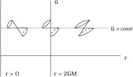
|
The surface r = 2GM, while being locally perfectly
regular, globally
functions as a point of no return - once a test particle dips
below it, it can never come back. For this reason r = 2GM
is known as the event horizon; no event at r ![]() 2GM can influence any
other event at r > 2GM. Notice that the event horizon
is a null surface,
not a timelike one. Notice also that since nothing can escape the
event horizon, it is impossible for us to "see inside" - thus the
name black hole.
2GM can influence any
other event at r > 2GM. Notice that the event horizon
is a null surface,
not a timelike one. Notice also that since nothing can escape the
event horizon, it is impossible for us to "see inside" - thus the
name black hole.
Let's consider what we have done. Acting under the suspicion that
our coordinates may not have been good for the entire manifold, we
have changed from our original coordinate t to the new one ![]() ,
which has the nice property that if we decrease r along a radial
curve null curve
,
which has the nice property that if we decrease r along a radial
curve null curve
![]() = constant, we go right through the
event horizon without any problems. (Indeed, a local observer actually
making the trip would not necessarily know when the event horizon had
been crossed - the local geometry is
no different than anywhere else.) We therefore
conclude that our suspicion was correct and our initial coordinate
system didn't do a good job of covering the entire manifold. The region
r
= constant, we go right through the
event horizon without any problems. (Indeed, a local observer actually
making the trip would not necessarily know when the event horizon had
been crossed - the local geometry is
no different than anywhere else.) We therefore
conclude that our suspicion was correct and our initial coordinate
system didn't do a good job of covering the entire manifold. The region
r ![]() 2GM should certainly be included in our
spacetime, since
physical particles can easily reach there and pass through. However,
there is no guarantee that we are finished; perhaps there are other
directions in which we can extend our manifold.
2GM should certainly be included in our
spacetime, since
physical particles can easily reach there and pass through. However,
there is no guarantee that we are finished; perhaps there are other
directions in which we can extend our manifold.
In fact there are. Notice that in the
(![]() , r) coordinate
system we can cross the event horizon on future-directed paths, but
not on past-directed ones. This seems unreasonable, since we started
with a time-independent solution. But we could have chosen
, r) coordinate
system we can cross the event horizon on future-directed paths, but
not on past-directed ones. This seems unreasonable, since we started
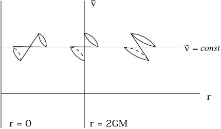
with a time-independent solution. But we could have chosen ![]() instead of
instead of ![]() , in which case the metric would have been
, in which case the metric would have been
| (7.72) |
Now we can once again pass through the event horizon, but this time only along past-directed curves.
|
This is perhaps a surprise: we can consistently follow either
future-directed or past-directed curves through r = 2GM,
but we
arrive at different places. It was actually to be expected, since
from the definitions (7.68), if we keep ![]() constant and decrease
r we must have
t
constant and decrease
r we must have
t ![]() +
+ ![]() , while if we keep
, while if we keep
![]() constant and decrease r we must have
t
constant and decrease r we must have
t ![]() -
- ![]() .
(The tortoise coordinate r* goes to -
.
(The tortoise coordinate r* goes to - ![]() as
r
as
r ![]() 2GM.)
So we have extended spacetime in two different directions, one to
the future and one to the past.
2GM.)
So we have extended spacetime in two different directions, one to
the future and one to the past.
The next step would be to follow spacelike geodesics to see if we
would uncover still more regions. The answer is yes, we would reach
yet another piece of the spacetime, but let's shortcut the process by
defining coordinates that are good all over. A first guess might be to
use both ![]() and
and ![]() at once (in place of t and r),
which leads to
at once (in place of t and r),
which leads to
| (7.73) |
with r defined implicitly in terms of ![]() and
and ![]() by
by
| (7.74) |
We have actually re-introduced the degeneracy with which we started
out; in these coordinates r = 2GM is "infinitely far away" (at
either
![]() = -
= - ![]() or
or
![]() = +
= + ![]() ). The thing to do
is to change to coordinates which pull these points into finite
coordinate values; a good choice is
). The thing to do
is to change to coordinates which pull these points into finite
coordinate values; a good choice is
| (7.75) |
which in terms of our original (t, r) system is
| (7.76) |
In the (u', v',![]() ,
,![]() ) system the Schwarzschild metric is
) system the Schwarzschild metric is
| (7.77) |
Finally the nonsingular nature of r = 2GM becomes completely manifest; in this form none of the metric coefficients behave in any special way at the event horizon.
Both u' and v' are null coordinates, in the sense that their
partial derivatives
![]() /
/![]() u' and
u' and
![]() /
/![]() v'
are null vectors. There is nothing wrong with this, since the
collection of four partial derivative vectors (two null and two
spacelike) in this system serve as a perfectly good basis for the
tangent space. Nevertheless, we are somewhat more comfortable working
in a system where one coordinate is timelike and the rest are
spacelike. We therefore define
v'
are null vectors. There is nothing wrong with this, since the
collection of four partial derivative vectors (two null and two
spacelike) in this system serve as a perfectly good basis for the
tangent space. Nevertheless, we are somewhat more comfortable working
in a system where one coordinate is timelike and the rest are
spacelike. We therefore define
| (7.78) |
and
| (7.79) |
in terms of which the metric becomes
| (7.80) |
where r is defined implicitly from
| (7.81) |
The coordinates
(v, u,![]() ,
,![]() ) are known as Kruskal
coordinates, or sometimes Kruskal-Szekres coordinates. Note that
v is the timelike coordinate.
) are known as Kruskal
coordinates, or sometimes Kruskal-Szekres coordinates. Note that
v is the timelike coordinate.
The Kruskal coordinates have a number of miraculous properties. Like the (t, r*) coordinates, the radial null curves look like they do in flat space:
| (7.82) |
Unlike the (t, r*) coordinates, however, the event horizon r = 2GM is not infinitely far away; in fact it is defined by

| (7.83) |
consistent with it being a null surface. More generally, we can consider the surfaces r = constant. From (7.81) these satisfy
| (7.84) |
Thus, they appear as hyperbolae in the u-v plane. Furthermore, the surfaces of constant t are given by
| (7.85) |
which defines straight lines through the origin with slope
tanh(t/4GM). Note that as
t ![]() ±
±![]() this
becomes the same as (7.83); therefore these surfaces are the
same as r = 2GM.
this
becomes the same as (7.83); therefore these surfaces are the
same as r = 2GM.
Now, our coordinates (v, u) should be allowed to
range over every value they can take without hitting the real
singularity at r = 2GM; the allowed region is therefore
- ![]()
![]() u
u ![]()
![]() and
v2 < u2 + 1. We can now draw
a spacetime diagram in the v-u plane (with
and
v2 < u2 + 1. We can now draw
a spacetime diagram in the v-u plane (with ![]() and
and ![]() suppressed), known as a "Kruskal diagram", which represents the
entire spacetime corresponding to the Schwarzschild metric.
suppressed), known as a "Kruskal diagram", which represents the
entire spacetime corresponding to the Schwarzschild metric.
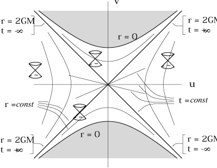
|
Each point on the diagram is a two-sphere.
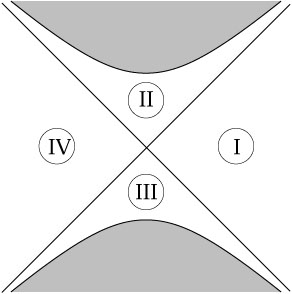
Our original coordinates (t, r) were only good for r > 2GM, which is only a part of the manifold portrayed on the Kruskal diagram. It is convenient to divide the diagram into four regions:
|
The region in which we started was region I; by following future-directed null rays we reached region II, and by following past-directed null rays we reached region III. If we had explored spacelike geodesics, we would have been led to region IV. The definitions (7.78) and (7.79) which relate (u, v) to (t, r) are really only good in region I; in the other regions it is necessary to introduce appropriate minus signs to prevent the coordinates from becoming imaginary.
Having extended the Schwarzschild geometry as far as it will go, we have described a remarkable spacetime. Region II, of course, is what we think of as the black hole. Once anything travels from region I into II, it can never return. In fact, every future-directed path in region II ends up hitting the singularity at r = 0; once you enter the event horizon, you are utterly doomed. This is worth stressing; not only can you not escape back to region I, you cannot even stop yourself from moving in the direction of decreasing r, since this is simply the timelike direction. (This could have been seen in our original coordinate system; for r < 2GM, t becomes spacelike and r becomes timelike.) Thus you can no more stop moving toward the singularity than you can stop getting older. Since proper time is maximized along a geodesic, you will live the longest if you don't struggle, but just relax as you approach the singularity. Not that you will have long to relax. (Nor that the voyage will be very relaxing; as you approach the singularity the tidal forces become infinite. As you fall toward the singularity your feet and head will be pulled apart from each other, while your torso is squeezed to infinitesimal thinness. The grisly demise of an astrophysicist falling into a black hole is detailed in Misner, Thorne, and Wheeler, section 32.6. Note that they use orthonormal frames [not that it makes the trip any more enjoyable].)
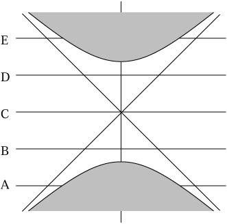
Regions III and IV might be somewhat unexpected. Region III is simply the time-reverse of region II, a part of spacetime from which things can escape to us, while we can never get there. It can be thought of as a "white hole." There is a singularity in the past, out of which the universe appears to spring. The boundary of region III is sometimes called the past event horizon, while the boundary of region II is called the future event horizon. Region IV, meanwhile, cannot be reached from our region I either forward or backward in time (nor can anybody from over there reach us). It is another asymptotically flat region of spacetime, a mirror image of ours. It can be thought of as being connected to region I by a "wormhole," a neck-like configuration joining two distinct regions. Consider slicing up the Kruskal diagram into spacelike surfaces of constant v:
|
Now we can draw pictures of each slice, restoring one of the angular coordinates for clarity:

|
So the Schwarzschild geometry really describes two asymptotically flat regions which reach toward each other, join together via a wormhole for a while, and then disconnect. But the wormhole closes up too quickly for any timelike observer to cross it from one region into the next.
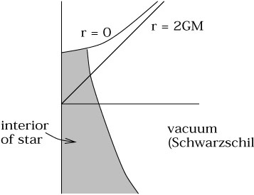
It might seem somewhat implausible, this story about two separate spacetimes reaching toward each other for a while and then letting go. In fact, it is not expected to happen in the real world, since the Schwarzschild metric does not accurately model the entire universe. Remember that it is only valid in vacuum, for example outside a star. If the star has a radius larger than 2GM, we need never worry about any event horizons at all. But we believe that there are stars which collapse under their own gravitational pull, shrinking down to below r = 2GM and further into a singularity, resulting in a black hole. There is no need for a white hole, however, because the past of such a spacetime looks nothing like that of the full Schwarzschild solution. Roughly, a Kruskal-like diagram for stellar collapse would look like the following:
|
The shaded region is not described by Schwarzschild, so there is no need to fret about white holes and wormholes.
While we are on the subject, we can say something about the formation of astrophysical black holes from massive stars. The life of a star is a constant struggle between the inward pull of gravity and the outward push of pressure. When the star is burning nuclear fuel at its core, the pressure comes from the heat produced by this burning. (We should put "burning" in quotes, since nuclear fusion is unrelated to oxidation.) When the fuel is used up, the temperature declines and the star begins to shrink as gravity starts winning the struggle. Eventually this process is stopped when the electrons are pushed so close together that they resist further compression simply on the basis of the Pauli exclusion principle (no two fermions can be in the same state). The resulting object is called a white dwarf. If the mass is sufficiently high, however, even the electron degeneracy pressure is not enough, and the electrons will combine with the protons in a dramatic phase transition. The result is a neutron star, which consists of almost entirely neutrons (although the insides of neutron stars are not understood terribly well). Since the conditions at the center of a neutron star are very different from those on earth, we do not have a perfect understanding of the equation of state. Nevertheless, we believe that a sufficiently massive neutron star will itself be unable to resist the pull of gravity, and will continue to collapse. Since a fluid of neutrons is the densest material of which we can presently conceive, it is believed that the inevitable outcome of such a collapse is a black hole.
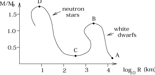
The process is summarized in the following diagram of radius vs. mass:
|
The point of the diagram is that, for any given mass M, the star will decrease in radius until it hits the line. White dwarfs are found between points A and B, and neutron stars between points C and D. Point B is at a height of somewhat less than 1.4 solar masses; the height of D is less certain, but probably less than 2 solar masses. The process of collapse is complicated, and during the evolution the star can lose or gain mass, so the endpoint of any given star is hard to predict. Nevertheless white dwarfs are all over the place, neutron stars are not uncommon, and there are a number of systems which are strongly believed to contain black holes. (Of course, you can't directly see the black hole. What you can see is radiation from matter accreting onto the hole, which heats up as it gets closer and emits radiation.)
We have seen that the Kruskal coordinate system provides a very useful representation of the Schwarzschild geometry. Before moving on to other types of black holes, we will introduce one more way of thinking about this spacetime, the Penrose (or Carter-Penrose, or conformal) diagram. The idea is to do a conformal transformation which brings the entire manifold onto a compact region such that we can fit the spacetime on a piece of paper.
Let's begin with Minkowski space, to see how the technique works. The metric in polar coordinates is
| (7.86) |
Nothing unusual will happen to the
![]() ,
,![]() coordinates, but
we will want to keep careful track of the ranges of the other two
coordinates. In this case of course we have
coordinates, but
we will want to keep careful track of the ranges of the other two
coordinates. In this case of course we have

| (7.87) |
Technically the worldline r = 0 represents a coordinate singularity and should be covered by a different patch, but we all know what is going on so we'll just act like r = 0 is well-behaved.
Our task is made somewhat easier if we switch to null coordinates:
| (7.88) |
with corresponding ranges given by
| (7.89) |

|
These ranges are as portrayed in the figure, on which each point represents a 2-sphere of radius r = u - v. The metric in these coordinates is given by

| (7.90) |
We now want to change to coordinates in which "infinity" takes on a finite coordinate value. A good choice is
| (7.91) |
|
The ranges are now
| (7.92) |
To get the metric, use

| (7.93) |
and
| (7.94) |
and likewise for v. We are led to
| (7.95) |
Meanwhile,
| (7.96) |
Therefore, the Minkowski metric in these coordinates is

| (7.97) |
This has a certain appeal, since the metric appears as a fairly
simple expression multiplied by an overall factor. We can make it
even better by transforming back to a timelike coordinate ![]() and a spacelike (radial) coordinate
and a spacelike (radial) coordinate ![]() , via
, via

| (7.98) |
with ranges

| (7.99) |
Now the metric is
| (7.100) |
where
| (7.101) |
The Minkowski metric may therefore be thought of as related by a conformal transformation to the "unphysical" metric
| (7.102) |
This describes the manifold
![]() × S3, where the 3-sphere is
maximally symmetric and static. There is curvature in this metric,
and it is not a solution to the vacuum Einstein's equations.
This shouldn't bother us, since
it is unphysical; the true physical metric, obtained by a conformal
transformation, is simply flat spacetime. In fact this metric is
that of the "Einstein static universe," a static (but unstable)
solution to Einstein's equations with a perfect fluid and a cosmological
constant. Of course, the full range of coordinates on
× S3, where the 3-sphere is
maximally symmetric and static. There is curvature in this metric,
and it is not a solution to the vacuum Einstein's equations.
This shouldn't bother us, since
it is unphysical; the true physical metric, obtained by a conformal
transformation, is simply flat spacetime. In fact this metric is
that of the "Einstein static universe," a static (but unstable)
solution to Einstein's equations with a perfect fluid and a cosmological
constant. Of course, the full range of coordinates on
![]() × S3
would usually be -
× S3
would usually be - ![]() <
< ![]() < +
< + ![]() ,
0
,
0 ![]()
![]()
![]()
![]() ,
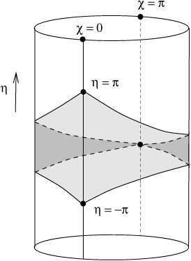
while Minkowski space is mapped into the subspace defined by (7.99).
The entire
,
while Minkowski space is mapped into the subspace defined by (7.99).
The entire
![]() × S3 can be drawn as a
cylinder, in which each
circle is a three-sphere, as shown on the next page.
× S3 can be drawn as a
cylinder, in which each
circle is a three-sphere, as shown on the next page.
|
The shaded region represents Minkowski space. Note that
each point
(![]() ,
,![]() ) on this cylinder is half of a two-sphere, where
the other half is the point
(
) on this cylinder is half of a two-sphere, where
the other half is the point
(![]() , -
, - ![]() ). We can unroll the
shaded region to portray Minkowski space as a triangle, as shown
in the figure.
). We can unroll the
shaded region to portray Minkowski space as a triangle, as shown
in the figure.
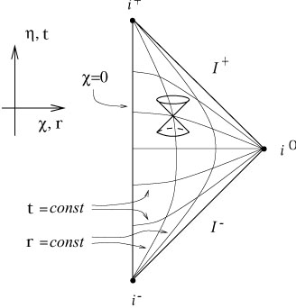
|
The is the Penrose diagram. Each point represents a two-sphere.
In fact Minkowski space is only the interior of the above
diagram (including ![]() = 0); the boundaries are not part of the
original spacetime. Together they are referred to as conformal
infinity. The structure of the Penrose diagram allows us to subdivide
conformal infinity into
a few different regions:
= 0); the boundaries are not part of the
original spacetime. Together they are referred to as conformal
infinity. The structure of the Penrose diagram allows us to subdivide
conformal infinity into
a few different regions:
|
(![]() + and
+ and
![]() - are pronounced as "scri-plus" and
"scri-minus", respectively.) Note that i+,
i0, and i- are
actually points, since
- are pronounced as "scri-plus" and
"scri-minus", respectively.) Note that i+,
i0, and i- are
actually points, since ![]() = 0 and
= 0 and ![]() =
= ![]() are the north and
south poles of S3. Meanwhile
are the north and
south poles of S3. Meanwhile
![]() + and
+ and
![]() - are
actually null surfaces, with the topology of
- are
actually null surfaces, with the topology of
![]() × S2.
× S2.
There are a number of important features of the Penrose diagram for
Minkowski spacetime. The points i+, and
i- can be thought of
as the limits of spacelike surfaces whose normals are timelike;
conversely, i0 can be thought of as the limit of
timelike surfaces
whose normals are spacelike. Radial null geodesics are at
±45° in the diagram.
All timelike geodesics begin at i-
and end at i+; all null geodesics begin at
![]() - and end at
- and end at
![]() +; all spacelike geodesics both begin and
end at i0.
On the other hand, there can be non-geodesic timelike curves that
end at null infinity (if they become "asymptotically null").
+; all spacelike geodesics both begin and
end at i0.
On the other hand, there can be non-geodesic timelike curves that
end at null infinity (if they become "asymptotically null").
It is nice to be able to fit all of Minkowski space on a small piece of paper, but we don't really learn much that we didn't already know. Penrose diagrams are more useful when we want to represent slightly more interesting spacetimes, such as those for black holes. The original use of Penrose diagrams was to compare spacetimes to Minkowski space "at infinity" - the rigorous definition of "asymptotically flat" is basically that a spacetime has a conformal infinity just like Minkowski space. We will not pursue these issues in detail, but instead turn directly to analysis of the Penrose diagram for a Schwarzschild black hole.
We will not go through the necessary manipulations in detail, since they parallel the Minkowski case with considerable additional algebraic complexity. We would start with the null version of the Kruskal coordinates, in which the metric takes the form
| (7.103) |
where r is defined implicitly via
| (7.104) |
Then essentially the same transformation as was used in flat spacetime suffices to bring infinity into finite coordinate values:
| (7.105) |
with ranges
|
The (u", v") part of the metric (that is, at constant angular coordinates) is now conformally related to Minkowski space. In the new coordinates the singularities at r = 0 are straight lines that stretch from timelike infinity in one asymptotic region to timelike infinity in the other. The Penrose diagram for the maximally extended Schwarzschild solution thus looks like this:

|
The only real subtlety about this diagram is the necessity to understand that i+ and i- are distinct from r = 0 (there are plenty of timelike paths that do not hit the singularity). Notice also that the structure of conformal infinity is just like that of Minkowski space, consistent with the claim that Schwarzschild is asymptotically flat. Also, the Penrose diagram for a collapsing star that forms a black hole is what you might expect, as shown on the next page.

|
Once again the Penrose diagrams for these spacetimes don't really tell us anything we didn't already know; their usefulness will become evident when we consider more general black holes. In principle there could be a wide variety of types of black holes, depending on the process by which they were formed. Surprisingly, however, this turns out not to be the case; no matter how a black hole is formed, it settles down (fairly quickly) into a state which is characterized only by the mass, charge, and angular momentum. This property, which must be demonstrated individually for the various types of fields which one might imagine go into the construction of the hole, is often stated as "black holes have no hair." You can demonstrate, for example, that a hole which is formed from an initially inhomogeneous collapse "shakes off" any lumpiness by emitting gravitational radiation. This is an example of a "no-hair theorem." If we are interested in the form of the black hole after it has settled down, we thus need only to concern ourselves with charged and rotating holes. In both cases there exist exact solutions for the metric, which we can examine closely.
But first let's take a brief detour to the world of black
hole evaporation.
It is strange to think of a black hole "evaporating," but in
the real world black holes aren't truly black - they radiate
energy as if they were a blackbody of temperature
T = ![]() /8
/8![]() kGM, where M is the mass of the hole and
k is Boltzmann's
constant. The derivation of this effect, known as Hawking
radiation, involves the use of quantum field theory in curved
spacetime and is way outside our scope right now. The informal
idea is nevertheless understandable.
kGM, where M is the mass of the hole and
k is Boltzmann's
constant. The derivation of this effect, known as Hawking
radiation, involves the use of quantum field theory in curved
spacetime and is way outside our scope right now. The informal
idea is nevertheless understandable.
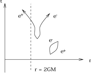
|
In quantum field theory there are "vacuum fluctuations" - the spontaneous creation and annihilation of particle/antiparticle pairs in empty space. These fluctuations are precisely analogous to the zero-point fluctuations of a simple harmonic oscillator. Normally such fluctuations are impossible to detect, since they average out to give zero total energy (although nobody knows why; that's the cosmological constant problem). In the presence of an event horizon, though, occasionally one member of a virtual pair will fall into the black hole while its partner escapes to infinity. The particle that reaches infinity will have to have a positive energy, but the total energy is conserved; therefore the black hole has to lose mass. (If you like you can think of the particle that falls in as having a negative mass.) We see the escaping particles as Hawking radiation. It's not a very big effect, and the temperature goes down as the mass goes up, so for black holes of mass comparable to the sun it is completely negligible. Still, in principle the black hole could lose all of its mass to Hawking radiation, and shrink to nothing in the process. The relevant Penrose diagram might look like this:

|
On the other hand, it might not. The problem with this diagram is that "information is lost" - if we draw a spacelike surface to the past of the singularity and evolve it into the future, part of it ends up crashing into the singularity and being destroyed. As a result the radiation itself contains less information than the information that was originally in the spacetime. (This is the worse than a lack of hair on the black hole. It's one thing to think that information has been trapped inside the event horizon, but it is more worrisome to think that it has disappeared entirely.) But such a process violates the conservation of information that is implicit in both general relativity and quantum field theory, the two theories that led to the prediction. This paradox is considered a big deal these days, and there are a number of efforts to understand how the information can somehow be retrieved. A currently popular explanation relies on string theory, and basically says that black holes have a lot of hair, in the form of virtual stringy states living near the event horizon. I hope you will not be disappointed to hear that we won't look at this very closely; but you should know what the problem is and that it is an area of active research these days.
With that out of our system, we now turn to electrically charged black holes. These seem at first like reasonable enough objects, since there is certainly nothing to stop us from throwing some net charge into a previously uncharged black hole. In an astrophysical situation, however, the total amount of charge is expected to be very small, especially when compared with the mass (in terms of the relative gravitational effects). Nevertheless, charged black holes provide a useful testing ground for various thought experiments, so they are worth our consideration.
In this case the full spherical symmetry of the problem is still present; we know therefore that we can write the metric as

| (7.106) |
Now, however, we are no longer in vacuum, since the hole will have a nonzero electromagnetic field, which in turn acts as a source of energy-momentum. The energy-momentum tensor for electromagnetism is given by
| (7.107) |
where F![]()
![]() is the electromagnetic field strength
tensor. Since we have spherical symmetry, the most general field
strength tensor will have components
is the electromagnetic field strength
tensor. Since we have spherical symmetry, the most general field
strength tensor will have components
| (7.108) |
where f (r, t) and g(r, t) are
some functions to be determined
by the field equations, and components not written are zero.
Ftr corresponds to a radial electric field, while
F![]()
![]() corresponds to a radial magnetic field. (For those of you wondering
about the
sin
corresponds to a radial magnetic field. (For those of you wondering
about the
sin![]() , recall that the thing which should be independent
of
, recall that the thing which should be independent
of ![]() and
and ![]() is the radial component of the magnetic field,
Br =
is the radial component of the magnetic field,
Br = ![]() F
F![]()
![]() . For a spherically symmetric metric,
. For a spherically symmetric metric,
![]() =
= ![]()
![]() is proportional to
(sin
is proportional to
(sin![]() )-1, so we want a factor of
sin
)-1, so we want a factor of
sin![]() in F
in F![]()
![]() .) The field equations in this case are
both Einstein's equations and Maxwell's equations:
.) The field equations in this case are
both Einstein's equations and Maxwell's equations:
| (7.109) |
The two sets are coupled together, since the electromagnetic field strength tensor enters Einstein's equations through the energy-momentum tensor, while the metric enters explicitly into Maxwell's equations.
The difficulties are not insurmountable, however, and a procedure similar to the one we followed for the vacuum case leads to a solution for the charged case as well. We will not go through the steps explicitly, but merely quote the final answer. The solution is known as the Reissner-Nordstrøm metric, and is given by
| (7.110) |
where
| (7.111) |
In this expression, M is once again interpreted as the mass of the hole; q is the total electric charge, and p is the total magnetic charge. Isolated magnetic charges (monopoles) have never been observed in nature, but that doesn't stop us from writing down the metric that they would produce if they did exist. There are good theoretical reasons to think that monopoles exist, but are extremely rare. (Of course, there is also the possibility that a black hole could have magnetic charge even if there aren't any monopoles.) In fact the electric and magnetic charges enter the metric in the same way, so we are not introducing any additional complications by keeping p in our expressions. The electromagnetic fields associated with this solution are given by
| (7.112) |
Conservatives are welcome to set p = 0 if they like.
The structure of singularities and event horizons is more
complicated in this metric than it was in Schwarzschild,
due to the extra term in the function ![]() (r) (which can
be thought of as measuring "how much the light cones tip over").
One thing remains the same: at r = 0 there is a true curvature
singularity (as could be checked by computing the curvature
scalar
R
(r) (which can
be thought of as measuring "how much the light cones tip over").
One thing remains the same: at r = 0 there is a true curvature
singularity (as could be checked by computing the curvature
scalar
R![]()
![]()
![]()
![]() R
R![]()
![]()
![]()
![]() ).
Meanwhile,
the equivalent of r = 2GM will be the radius where
).
Meanwhile,
the equivalent of r = 2GM will be the radius where ![]() vanishes. This will occur at
vanishes. This will occur at
| (7.113) |
This might constitute two, one, or zero solutions, depending on the relative values of GM2 and p2 + q2. We therefore consider each case separately.
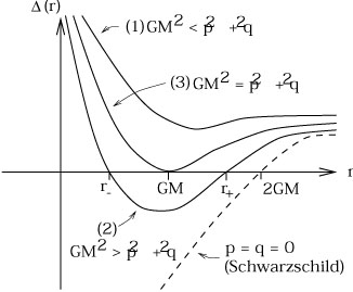
|
Case One - GM2 < p2 + q2
In this case the coefficient ![]() is always positive (never zero),
and the metric is completely regular in the (t, r,
is always positive (never zero),
and the metric is completely regular in the (t, r, ![]() ,
,![]() )
coordinates all the way down to r = 0. The coordinate t is
always timelike, and r is always spacelike. But there still
is the singularity at r = 0, which is now a timelike line.
Since there is no event horizon, there is no obstruction
to an observer travelling to the singularity and returning
to report on what was observed. This is known as a
naked singularity, one which is not shielded by an
horizon. A careful analysis of the geodesics reveals, however,
that the singularity is "repulsive" - timelike geodesics
never intersect r = 0, instead they approach and then reverse
course and move away. (Null geodesics can reach the singularity,
as can non-geodesic timelike curves.)
)
coordinates all the way down to r = 0. The coordinate t is
always timelike, and r is always spacelike. But there still
is the singularity at r = 0, which is now a timelike line.
Since there is no event horizon, there is no obstruction
to an observer travelling to the singularity and returning
to report on what was observed. This is known as a
naked singularity, one which is not shielded by an
horizon. A careful analysis of the geodesics reveals, however,
that the singularity is "repulsive" - timelike geodesics
never intersect r = 0, instead they approach and then reverse
course and move away. (Null geodesics can reach the singularity,
as can non-geodesic timelike curves.)
As
r ![]()
![]() the solution approaches flat spacetime,
and as we have just seen the causal structure is "normal" everywhere.
The Penrose diagram will therefore be just like that of Minkowski
space, except that now r = 0 is a singularity.
the solution approaches flat spacetime,
and as we have just seen the causal structure is "normal" everywhere.
The Penrose diagram will therefore be just like that of Minkowski
space, except that now r = 0 is a singularity.
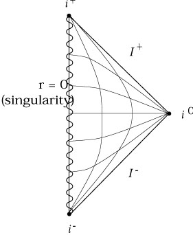
|
The nakedness of the singularity offends our sense of decency, as well as the cosmic censorship conjecture, which roughly states that the gravitational collapse of physical matter configurations will never produce a naked singularity. (Of course, it's just a conjecture, and it may not be right; there are some claims from numerical simulations that collapse of spindle-like configurations can lead to naked singularities.) In fact, we should not ever expect to find a black hole with GM2 < p2 + q2 as the result of gravitational collapse. Roughly speaking, this condition states that the total energy of the hole is less than the contribution to the energy from the electromagnetic fields alone - that is, the mass of the matter which carried the charge would have had to be negative. This solution is therefore generally considered to be unphysical. Notice also that there are not good Cauchy surfaces (spacelike slices for which every inextendible timelike line intersects them) in this spacetime, since timelike lines can begin and end at the singularity.
Case Two - GM2 > p2 + q2
This is the situation which we expect to apply in real gravitational
collapse; the energy in the electromagnetic field is less than the
total energy. In this case the metric coefficient ![]() (r) is
positive at large r and small r, and negative inside the two
vanishing points
r± = GM±
(r) is
positive at large r and small r, and negative inside the two
vanishing points
r± = GM±![]() . The
metric has coordinate singularities at both r+ and
r-; in
both cases these could be removed by a change of coordinates as we
did with Schwarzschild.
. The
metric has coordinate singularities at both r+ and
r-; in
both cases these could be removed by a change of coordinates as we
did with Schwarzschild.
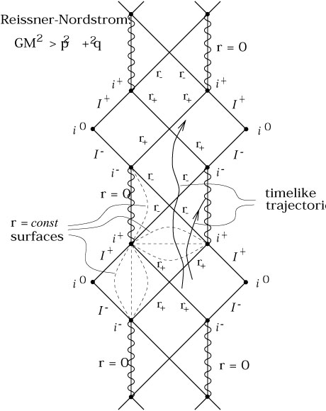
|
The surfaces defined by r = r± are both null, and in fact they are event horizons (in a sense we will make precise in a moment). The singularity at r = 0 is a timelike line (not a spacelike surface as in Schwarzschild). If you are an observer falling into the black hole from far away, r+ is just like 2GM in the Schwarzschild metric; at this radius r switches from being a spacelike coordinate to a timelike coordinate, and you necessarily move in the direction of decreasing r. Witnesses outside the black hole also see the same phenomena that they would outside an uncharged hole - the infalling observer is seen to move more and more slowly, and is increasingly redshifted.
But the inevitable fall from r+ to ever-decreasing radii only lasts until you reach the null surface r = r-, where r switches back to being a spacelike coordinate and the motion in the direction of decreasing r can be arrested. Therefore you do not have to hit the singularity at r = 0; this is to be expected, since r = 0 is a timelike line (and therefore not necessarily in your future). In fact you can choose either to continue on to r = 0, or begin to move in the direction of increasing r back through the null surface at r = r-. Then r will once again be a timelike coordinate, but with reversed orientation; you are forced to move in the direction of increasing r. You will eventually be spit out past r = r+ once more, which is like emerging from a white hole into the rest of the universe. From here you can choose to go back into the black hole - this time, a different hole than the one you entered in the first place - and repeat the voyage as many times as you like. This little story corresponds to the accompanying Penrose diagram, which of course can be derived more rigorously by choosing appropriate coordinates and analytically extending the Reissner-Nordstrøm metric as far as it will go.
How much of this is science, as opposed to science fiction? Probably not much. If you think about the world as seen from an observer inside the black hole who is about to cross the event horizon at r-, you will notice that they can look back in time to see the entire history of the external (asymptotically flat) universe, at least as seen from the black hole. But they see this (infinitely long) history in a finite amount of their proper time - thus, any signal that gets to them as they approach r- is infinitely blueshifted. Therefore it is reasonable to believe (although I know of no proof) that any non-spherically symmetric perturbation that comes into a Reissner-Nordstrøm black hole will violently disturb the geometry we have described. It's hard to say what the actual geometry will look like, but there is no very good reason to believe that it must contain an infinite number of asymptotically flat regions connecting to each other via various wormholes.
Case Three - GM2 = p2 + q2
This case is known as the extreme Reissner-Nordstrøm solution (or simply "extremal black hole"). The mass is exactly balanced in some sense by the charge - you can construct exact solutions consisting of several extremal black holes which remain stationary with respect to each other for all time. On the one hand the extremal hole is an amusing theoretical toy; these solutions are often examined in studies of the information loss paradox, and the role of black holes in quantum gravity. On the other hand it appears very unstable, since adding just a little bit of matter will bring it to Case Two.
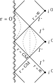
|
The extremal black holes have
![]() (r) = 0 at a single radius,
r = GM. This does represent an event horizon, but the r
coordinate is never timelike; it becomes null at r = GM,
but is
spacelike on either side. The singularity at r = 0 is a
timelike line, as in the other cases. So for this black hole
you can again avoid the singularity and continue to move to the
future to extra copies of the asymptotically flat region, but
the singularity is always "to the left." The Penrose diagram
is as shown.
(r) = 0 at a single radius,
r = GM. This does represent an event horizon, but the r
coordinate is never timelike; it becomes null at r = GM,
but is
spacelike on either side. The singularity at r = 0 is a
timelike line, as in the other cases. So for this black hole
you can again avoid the singularity and continue to move to the
future to extra copies of the asymptotically flat region, but
the singularity is always "to the left." The Penrose diagram
is as shown.
We could of course go into a good deal more detail about the charged solutions, but let's instead move on to spinning black holes. It is much more difficult to find the exact solution for the metric in this case, since we have given up on spherical symmetry. To begin with all that is present is axial symmetry (around the axis of rotation), but we can also ask for stationary solutions (a timelike Killing vector). Although the Schwarzschild and Reissner-Nordstrøm solutions were discovered soon after general relativity was invented, the solution for a rotating black hole was found by Kerr only in 1963. His result, the Kerr metric, is given by the following mess:

| (7.114) |
where
| (7.115) |
and
| (7.116) |
Here a measures the rotation of the hole and M is the mass. It is straightforward to include electric and magnetic charges q and p, simply by replacing 2GMr with 2GMr - (q2 + p2) / G; the result is the Kerr-Newman metric. All of the interesting phenomena persist in the absence of charges, so we will set q = p = 0 from now on.
The coordinates
(t, r,![]() ,
,![]() ) are known as
Boyer-Lindquist coordinates. It is straightforward to check that
as a
) are known as
Boyer-Lindquist coordinates. It is straightforward to check that
as a ![]() 0 they reduce to Schwarzschild coordinates. If
we keep a fixed and let
M
0 they reduce to Schwarzschild coordinates. If
we keep a fixed and let
M ![]() 0, however, we recover
flat spacetime but not in ordinary polar coordinates. The metric
becomes
0, however, we recover
flat spacetime but not in ordinary polar coordinates. The metric
becomes

| (7.117) |
and we recognize the spatial part of this as flat space in ellipsoidal coordinates.
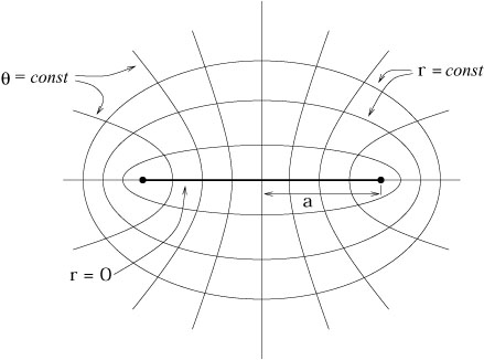
|
They are related to Cartesian coordinates in Euclidean 3-space by
| (7.118) |
There are two Killing vectors of the metric (7.114), both of
which are manifest; since the metric coefficients are independent
of t and ![]() , both
, both
![]() =
= ![]() and
and
![]() =
= ![]() are Killing
vectors. Of course
are Killing
vectors. Of course ![]() expresses the axial symmetry of the solution.
The vector
expresses the axial symmetry of the solution.
The vector ![]() is not orthogonal to t = constant
hypersurfaces,
and in fact is not orthogonal to any hypersurfaces at all;
hence this metric is stationary, but not static. (It's not changing
with time, but it is spinning.)
is not orthogonal to t = constant
hypersurfaces,
and in fact is not orthogonal to any hypersurfaces at all;
hence this metric is stationary, but not static. (It's not changing
with time, but it is spinning.)
What is more, the Kerr metric
also possesses something called a Killing tensor. This is
any symmetric (0, n) tensor
![]() which satisfies
which satisfies
| (7.119) |
Simple examples of Killing tensors are the metric itself, and symmetrized tensor products of Killing vectors. Just as a Killing vector implies a constant of geodesic motion, if there exists a Killing tensor then along a geodesic we will have
| (7.120) |
(Unlike Killing vectors, higher-rank Killing tensors do not correspond to symmetries of the metric.) In the Kerr geometry we can define the (0, 2) tensor
| (7.121) |
In this expression the two vectors l and n are given (with indices raised) by
| (7.122) |
Both vectors are null and satisfy

| (7.123) |
(For what it is worth, they are the "special null vectors" of the
Petrov classification for this spacetime.) With these definitions,
you can check for yourself that
![]() is a Killing tensor.
is a Killing tensor.
Let's think about the structure of the full Kerr solution. Singularities
seem to appear at both ![]() = 0 and
= 0 and ![]() = 0; let's turn our
attention first to
= 0; let's turn our
attention first to ![]() = 0. As in the Reissner-Nordstrøm
solution there are three possibilities:
G2M2 > a2,
G2M2 = a2, and
G2M2 < a2. The
last case features a naked singularity, and the extremal case
G2M2 = a2 is
unstable, just as in Reissner-Nordstrøm.
Since these cases are of less physical interest, and time is short,
we will concentrate on
G2M2 > a2. Then
there are two radii at
which
= 0. As in the Reissner-Nordstrøm
solution there are three possibilities:
G2M2 > a2,
G2M2 = a2, and
G2M2 < a2. The
last case features a naked singularity, and the extremal case
G2M2 = a2 is
unstable, just as in Reissner-Nordstrøm.
Since these cases are of less physical interest, and time is short,
we will concentrate on
G2M2 > a2. Then
there are two radii at
which ![]() vanishes, given by
vanishes, given by
| (7.124) |
Both radii are null surfaces which will turn out to be event horizons. The analysis of these surfaces proceeds in close analogy with the Reissner-Nordstrøm case; it is straightforward to find coordinates which extend through the horizons.
Besides the event horizons at r±, the Kerr
solution also
features an additional surface of interest. Recall that in the
spherically symmetric solutions, the "timelike" Killing vector
![]() =
= ![]() actually became null on the (outer) event
horizon, and spacelike inside. Checking to see where the
analogous thing happens for Kerr, we compute
actually became null on the (outer) event
horizon, and spacelike inside. Checking to see where the
analogous thing happens for Kerr, we compute
| (7.125) |
This does not vanish at the outer event horizon; in fact, at r =
r+
(where ![]() = 0), we have
= 0), we have
| (7.126) |
So the Killing vector is already spacelike at the outer horizon,
except at the north and south poles (![]() = 0) where it is null.
The locus of points where
= 0) where it is null.
The locus of points where
![]()
![]() = 0 is known as the
Killing horizon, and is given by
= 0 is known as the
Killing horizon, and is given by
| (7.127) |
while the outer event horizon is given by
| (7.128) |
There is thus a region in between these two surfaces, known as
the ergosphere. Inside the ergosphere, you must move in
the direction of the rotation of the black hole (the ![]() direction);
however, you can still towards or away from the event horizon
(and there is no trouble exiting the ergosphere).
It is evidently a place where interesting
things can happen even before you cross the horizon; more details
on this later.
direction);
however, you can still towards or away from the event horizon
(and there is no trouble exiting the ergosphere).
It is evidently a place where interesting
things can happen even before you cross the horizon; more details
on this later.
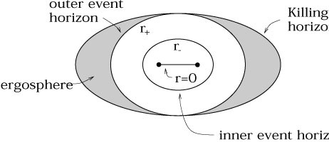
|
Before rushing to draw Penrose diagrams, we need to understand the
nature of the true curvature singularity; this does not occur at
r = 0 in this spacetime, but rather at ![]() = 0. Since
= 0. Since
![]() = r2 +
a2cos2
= r2 +
a2cos2![]() is the sum of two manifestly nonnegative
quantities, it can only vanish when both quantities are zero, or
is the sum of two manifestly nonnegative
quantities, it can only vanish when both quantities are zero, or
| (7.129) |
This seems like a funny result, but remember that r = 0 is not
a point in space, but a disk; the set of points r = 0,
![]() =
= ![]() /2
is actually the ring at the edge of this disk. The rotation
has "softened" the Schwarzschild singularity, spreading it out
over a ring.
/2
is actually the ring at the edge of this disk. The rotation
has "softened" the Schwarzschild singularity, spreading it out
over a ring.
What happens if you go inside the ring? A careful analytic
continuation (which we will not perform) would reveal that you
exit to another asymptotically flat spacetime, but not an identical
copy of the one you came from. The new spacetime is described
by the Kerr metric with r < 0. As a result, ![]() never vanishes
and there are no horizons. The Penrose diagram is much like that for
Reissner-Nordstrøm, except now you can pass through the singularity.
never vanishes
and there are no horizons. The Penrose diagram is much like that for
Reissner-Nordstrøm, except now you can pass through the singularity.
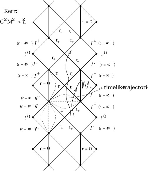
|
Not only do we have the usual strangeness of these distinct
asymptotically flat regions connected to ours through the black
hole, but the region near the ring singularity has additional
pathologies: closed timelike curves. If you consider trajectories
which wind around in ![]() while keeping
while keeping ![]() and t
constant and r a small negative value, the line element along such
a path is
and t
constant and r a small negative value, the line element along such
a path is
| (7.130) |
which is negative for small negative r. Since these paths are closed, they are obviously CTC's. You can therefore meet yourself in the past, with all that entails.
Of course, everything we say about the analytic extension of Kerr is subject to the same caveats we mentioned for Schwarzschild and Reissner-Nordstrøm; it is unlikely that realistic gravitational collapse leads to these bizarre spacetimes. It is nevertheless always useful to have exact solutions. Furthermore, for the Kerr metric there are strange things happening even if we stay outside the event horizon, to which we now turn.
We begin by considering more carefully the angular velocity of the
hole. Obviously the conventional definition of angular velocity
will have to be modified somewhat before we can apply it to something
as abstract as the metric of spacetime. Let us consider the fate
of a photon which is emitted in the ![]() direction at some
radius r in the equatorial plane (
direction at some
radius r in the equatorial plane (![]() =
= ![]() /2) of a Kerr black
hole. The instant it is emitted its momentum has no components in
the r or
/2) of a Kerr black
hole. The instant it is emitted its momentum has no components in
the r or ![]() direction, and therefore the condition that it
be null is
direction, and therefore the condition that it
be null is

| (7.131) |
This can be immediately solved to obtain
| (7.132) |
If we evaluate this quantity on the Killing horizon of the Kerr metric, we have gtt = 0, and the two solutions are
| (7.133) |
The nonzero solution has the same sign as a; we interpret this
as the photon moving around the hole in the same direction as the
hole's rotation. The zero solution means that the photon directed
against the hole's rotation doesn't move at all in this coordinate
system. (This isn't a full solution to the photon's trajectory, just
the statement that its instantaneous velocity is zero.) This is
an example of the "dragging of inertial frames" mentioned earlier.
The point of this exercise is to note that
massive particles, which must move more slowly than photons, are
necessarily dragged along with the hole's rotation once they are
inside the Killing horizon. This dragging continues as we approach
the outer event horizon at r+; we can define the
angular velocity
of the event horizon itself, ![]() , to be the minimum angular
velocity of a particle at the horizon. Directly from (7.132) we
find that
, to be the minimum angular
velocity of a particle at the horizon. Directly from (7.132) we
find that
| (7.134) |
Now let's turn to geodesic motion, which we know will be
simplified by considering the conserved quantities associated with
the Killing vectors
![]() =
= ![]() and
and
![]() =
= ![]() .
For the purposes at hand we can restrict our attention to massive
particles, for which we can work with the four-momentum
.
For the purposes at hand we can restrict our attention to massive
particles, for which we can work with the four-momentum

| (7.135) |
where m is the rest mass of the particle. Then we can take as our two conserved quantities the actual energy and angular momentum of the particle,
| (7.136) |
and

| (7.137) |
(These differ from our previous definitions for the conserved quantities, where E and L were taken to be the energy and angular momentum per unit mass. They are conserved either way, of course.)
The minus sign in the definition of E is there because at
infinity both ![]() and p
and p![]() are timelike, so their inner product is
negative,
but we want the energy to be positive. Inside the ergosphere, however,
are timelike, so their inner product is
negative,
but we want the energy to be positive. Inside the ergosphere, however,
![]() becomes spacelike; we can therefore imagine
particles for which
becomes spacelike; we can therefore imagine
particles for which
| (7.138) |
The extent to which this bothers us is ameliorated somewhat by the realization that all particles outside the Killing horizon must have positive energies; therefore a particle inside the ergosphere with negative energy must either remain on a geodesic inside the Killing horizon, or be accelerated until its energy is positive if it is to escape.
Still, this realization leads to a way to extract energy from a
rotating black hole; the method is known as the Penrose process.
The idea is simple; starting from outside the ergosphere, you arm
yourself with a large rock and leap toward the black hole. If we
call the four-momentum of the (you + rock) system
p(0)![]() , then
the energy
E(0) = -
, then
the energy
E(0) = - ![]() p(0)
p(0)![]() is certainly positive,
and conserved as you move along your geodesic. Once you enter the
ergosphere, you hurl the rock with all your might, in a very
specific way. If we call your momentum
p(1)
is certainly positive,
and conserved as you move along your geodesic. Once you enter the
ergosphere, you hurl the rock with all your might, in a very
specific way. If we call your momentum
p(1)![]() and that of
the rock
p(2)
and that of
the rock
p(2)![]() , then at the instant you throw it we have
conservation of momentum just as in special relativity:
, then at the instant you throw it we have
conservation of momentum just as in special relativity:
| (7.139) |
Contracting with the Killing vector ![]() gives
gives
| (7.140) |
But, if we imagine that you are arbitrarily strong (and accurate), you can arrange your throw such that E(2) < 0, as per (7.158).
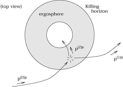
|
Furthermore, Penrose was able to show that you can arrange the initial trajectory and the throw such that afterwards you follow a geodesic trajectory back outside the Killing horizon into the external universe. Since your energy is conserved along the way, at the end we will have

| (7.141) |
Thus, you have emerged with more energy than you entered with.
There is no such thing as a free lunch; the energy you gained came from somewhere, and that somewhere is the black hole. In fact, the Penrose process extracts energy from the rotating black hole by decreasing its angular momentum; you have to throw the rock against the hole's rotation to get the trick to work. To see this more precisely, define a new Killing vector
| (7.142) |
On the outer horizon ![]() is null and tangent to
the horizon. (This can be seen from
is null and tangent to
the horizon. (This can be seen from
![]() =
= ![]() ,
,
![]() =
= ![]() , and the definition (7.134) of
, and the definition (7.134) of ![]() .)
The statement that the particle with momentum
p(2)
.)
The statement that the particle with momentum
p(2)![]() crosses the event horizon "moving forwards in time" is simply
crosses the event horizon "moving forwards in time" is simply

| (7.143) |
Plugging in the definitions of E and L, we see that this condition is equivalent to

| (7.144) |
Since we have arranged E(2) to be negative, and ![]() is positive, we see that the particle must have a negative
angular momentum - it is moving against the hole's rotation.
Once you have escaped the ergosphere and the rock has
fallen inside the event horizon, the mass and angular momentum
of the hole are what they used to be plus the negative
contributions of the rock:
is positive, we see that the particle must have a negative
angular momentum - it is moving against the hole's rotation.
Once you have escaped the ergosphere and the rock has
fallen inside the event horizon, the mass and angular momentum
of the hole are what they used to be plus the negative
contributions of the rock:

| (7.145) |
Here we have introduced the notation J for the angular momentum of the black hole; it is given by

| (7.146) |
We won't justify this, but you can look in Wald for an explanation. Then (7.144) becomes a limit on how much you can decrease the angular momentum:

| (7.147) |
If we exactly reach this limit, as the rock we throw in
becomes more and more null, we have the "ideal" process,
in which
![]() J =
J = ![]() M/
M/![]() .
.
We will now use these ideas to prove a powerful result: although you can use the Penrose process to extract energy from the black hole, you can never decrease the area of the event horizon. For a Kerr metric, one can go through a straightforward computation (projecting the metric and volume element and so on) to compute the area of the event horizon:
| (7.148) |
To show that this doesn't decrease, it is most convenient to work instead in terms of the irreducible mass of the black hole, defined by
| (7.149) |
We can differentiate to obtain, after a bit of work,
| (7.150) |
(I think I have the factors of G right, but it wouldn't hurt to check.) Then our limit (7.147) becomes

| (7.151) |
The irreducible mass can never be reduced; hence the name. It follows that the maximum amount of energy we can extract from a black hole before we slow its rotation to zero is
| (7.152) |
The result of this complete extraction is a Schwarzschild black hole of mass Mirr. It turns out that the best we can do is to start with an extreme Kerr black hole; then we can get out approximately 29% of its total energy.
The irreducibility of Mirr leads immediately to the fact that the area A can never decrease. From (7.149) and (7.150) we have
| (7.153) |
which can be recast as
| (7.154) |
where we have introduced
| (7.155) |
The quantity ![]() is known as the surface gravity
of the black hole.
is known as the surface gravity
of the black hole.
It was equations like (7.154) that first started people thinking about the relationship between black holes and thermodynamics. Consider the first law of thermodynamics,
| (7.156) |
It is natural to think of the term
![]()
![]() J as
"work" that we do on the black hole by throwing rocks into
it. Then the thermodynamic analogy begins to take shape
if we think of identifying the area A as the entropy
S, and the surface gravity
J as
"work" that we do on the black hole by throwing rocks into
it. Then the thermodynamic analogy begins to take shape
if we think of identifying the area A as the entropy
S, and the surface gravity ![]() as 8
as 8![]() G times the
temperature T. In fact, in the context of classical
general relativity the analogy is essentially perfect.
The "zeroth" law of thermodynamics states that in
thermal equilibrium the temperature is constant throughout
the system; the analogous statement for black holes is that
stationary black holes have constant surface gravity on
the entire horizon (true). As we have seen, the first
law (7.156) is equivalent to (7.154). The second law,
that entropy never decreases, is simply the statement that
the area of the horizon never decreases. Finally, the third
law is that it is impossible to achieve T = 0 in any
physical process, which should imply that it is impossible
to achieve
G times the
temperature T. In fact, in the context of classical
general relativity the analogy is essentially perfect.
The "zeroth" law of thermodynamics states that in
thermal equilibrium the temperature is constant throughout
the system; the analogous statement for black holes is that
stationary black holes have constant surface gravity on
the entire horizon (true). As we have seen, the first
law (7.156) is equivalent to (7.154). The second law,
that entropy never decreases, is simply the statement that
the area of the horizon never decreases. Finally, the third
law is that it is impossible to achieve T = 0 in any
physical process, which should imply that it is impossible
to achieve ![]() = 0 in any physical process. It turns
out that
= 0 in any physical process. It turns
out that ![]() = 0 corresponds to the extremal black
holes (either in Kerr or Reissner-Nordstrøm) - where
the naked singularities would appear. Somehow, then,
the third law is related to cosmic censorship.
= 0 corresponds to the extremal black
holes (either in Kerr or Reissner-Nordstrøm) - where
the naked singularities would appear. Somehow, then,
the third law is related to cosmic censorship.
The missing piece is that real thermodynamic bodies don't just sit there; they give off blackbody radiation with a spectrum that depends on their temperature. Black holes, it was thought before Hawking discovered his radiation, don't do that, since they're truly black. Historically, Bekenstein came up with the idea that black holes should really be honest black bodies, including the radiation at the appropriate temperature. This annoyed Hawking, who set out to prove him wrong, and ended up proving that there would be radiation after all. So the thermodynamic analogy is even better than we had any right to expect - although it is safe to say that nobody really knows why.