

Contemporary cosmological models are based on the idea that the
universe is pretty much the same everywhere - a stance sometimes
known as the Copernican principle. On the face of it, such
a claim seems preposterous; the center of the sun, for example,
bears little resemblance to the desolate cold of interstellar
space. But we take the Copernican principle to only apply on
the very largest scales, where local variations in density are
averaged over. Its validity on such scales is
manifested in a number of different observations, such as number counts
of galaxies and observations of diffuse X-ray and ![]() -ray
backgrounds, but is most clear in the 3° microwave background
radiation. Although we now know that the microwave background is not
perfectly smooth (and nobody ever expected that it was), the
deviations from regularity are on the order of 10-5 or less,
certainly an adequate basis for an approximate description of
spacetime on large scales.
-ray
backgrounds, but is most clear in the 3° microwave background
radiation. Although we now know that the microwave background is not
perfectly smooth (and nobody ever expected that it was), the
deviations from regularity are on the order of 10-5 or less,
certainly an adequate basis for an approximate description of
spacetime on large scales.
The Copernican principle is related to two more mathematically precise properties that a manifold might have: isotropy and homogeneity. Isotropy applies at some specific point in the space, and states that the space looks the same no matter what direction you look in. More formally, a manifold M is isotropic around a point p if, for any two vectors V and W in TpM, there is an isometry of M such that the pushforward of W under the isometry is parallel with V (not pushed forward). It is isotropy which is indicated by the observations of the microwave background.
Homogeneity is the statement that the metric is the same
throughout the space. In other words, given any two points p and
q in M, there is an isometry which takes p into
q. Note that there is no necessary relationship between homogeneity
and isotropy; a manifold can be homogeneous but nowhere isotropic
(such as
![]() × S2 in the usual metric), or it
can be isotropic
around a point without being homogeneous (such as a cone, which is
isotropic around its vertex but certainly not homogeneous). On the
other hand, if a space is isotropic everywhere then it is
homogeneous. (Likewise if it is isotropic around one point and
also homogeneous, it will be isotropic around every point.)
Since there is ample observational evidence for
isotropy, and the Copernican principle would have us believe that we
are not the center of the universe and therefore observers elsewhere
should also observe isotropy, we will henceforth assume both
homogeneity and isotropy.
× S2 in the usual metric), or it
can be isotropic
around a point without being homogeneous (such as a cone, which is
isotropic around its vertex but certainly not homogeneous). On the
other hand, if a space is isotropic everywhere then it is
homogeneous. (Likewise if it is isotropic around one point and
also homogeneous, it will be isotropic around every point.)
Since there is ample observational evidence for
isotropy, and the Copernican principle would have us believe that we
are not the center of the universe and therefore observers elsewhere
should also observe isotropy, we will henceforth assume both
homogeneity and isotropy.
There is one catch. When we look at distant galaxies, they appear
to be receding from us; the universe is apparently not static, but
changing with time. Therefore we begin construction of cosmological
models with the idea that the universe is homogeneous and isotropic
in space, but not in time. In general relativity this translates into
the statement that the universe can be foliated into spacelike slices
such that each slice is homogeneous and isotropic.
We therefore consider our spacetime to be
![]() ×
× ![]() , where
, where
![]() represents the time direction and
represents the time direction and ![]() is a homogeneous and
isotropic three-manifold. The usefulness of homogeneity and
isotropy is that they imply that
is a homogeneous and
isotropic three-manifold. The usefulness of homogeneity and
isotropy is that they imply that ![]() must be a maximally
symmetric space. (Think of isotropy as invariance under rotations,
and homogeneity as invariance under translations. Then homogeneity
and isotropy together imply that a space has its maximum possible
number of Killing vectors.) Therefore
we can take our metric to be of the form
must be a maximally
symmetric space. (Think of isotropy as invariance under rotations,
and homogeneity as invariance under translations. Then homogeneity
and isotropy together imply that a space has its maximum possible
number of Killing vectors.) Therefore
we can take our metric to be of the form

| (8.1) |
Here t is the timelike coordinate, and
(u1, u2, u3) are the
coordinates on ![]() ;
;
![]() is the maximally symmetric
metric on
is the maximally symmetric
metric on ![]() . This formula is a special case of (7.2), which we
used to derive the Schwarzschild metric, except we have scaled t
such that gtt = - 1. The function a(t)
is known as the
scale factor, and it tells us "how big" the spacelike
slice
. This formula is a special case of (7.2), which we
used to derive the Schwarzschild metric, except we have scaled t
such that gtt = - 1. The function a(t)
is known as the
scale factor, and it tells us "how big" the spacelike
slice ![]() is at the moment t. The coordinates used here,
in which the metric is free of cross terms
dt dui and the
spacelike components are proportional to a single function of t, are
known as comoving coordinates, and an observer who stays at constant
ui is also called "comoving". Only a comoving
observer will
think that the universe looks isotropic; in fact on Earth we are
not quite comoving, and as a result we see a dipole anisotropy in
the cosmic microwave background as a result of the conventional
Doppler effect.
is at the moment t. The coordinates used here,
in which the metric is free of cross terms
dt dui and the
spacelike components are proportional to a single function of t, are
known as comoving coordinates, and an observer who stays at constant
ui is also called "comoving". Only a comoving
observer will
think that the universe looks isotropic; in fact on Earth we are
not quite comoving, and as a result we see a dipole anisotropy in
the cosmic microwave background as a result of the conventional
Doppler effect.
Our interest is therefore in maximally symmetric Euclidean three-metrics
![]() . We know that maximally symmetric metrics
obey
. We know that maximally symmetric metrics
obey
| (8.2) |
where k is some constant, and we put a superscript (3) on
the Riemann tensor to remind us that it is associated with the
three-metric
![]() , not the metric of the entire spacetime.
The Ricci tensor is then
, not the metric of the entire spacetime.
The Ricci tensor is then

| (8.3) |
If the space is to be maximally symmetric, then it will certainly be spherically symmetric. We already know something about spherically symmetric spaces from our exploration of the Schwarzschild solution; the metric can be put in the form

| (8.4) |
The components of the Ricci tensor for such a metric can be obtained
from (7.16), the Ricci tensor for a spherically symmetric spacetime,
by setting ![]() = 0 and
= 0 and
![]()
![]() = 0, which gives
= 0, which gives
| (8.5) |
We set these proportional to the metric using (8.3), and can solve
for ![]() (r):
(r):
| (8.6) |
This gives us the following metric on spacetime:
| (8.7) |
This is the Robertson-Walker metric. We have not yet made use of Einstein's equations; those will determine the behavior of the scale factor a(t).
Note that the substitutions

| (8.8) |
leave (8.7) invariant. Therefore the only relevant parameter
is k/| k|, and there are three cases of interest: k
= - 1,
k = 0, and k = + 1. The k = - 1 case corresponds
to constant
negative curvature on ![]() , and is called open; the
k = 0 case corresponds to no curvature on
, and is called open; the
k = 0 case corresponds to no curvature on ![]() , and is called
flat; the k = + 1 case corresponds to positive curvature
on
, and is called
flat; the k = + 1 case corresponds to positive curvature
on ![]() ,
and is called closed.
,
and is called closed.
Let us examine each of these possibilities. For the flat case
k = 0 the metric on ![]() is
is
| (8.9) |
which is simply flat Euclidean space. Globally, it could describe
![]() or a more complicated manifold, such as the
three-torus S1 × S1 ×
S1. For the closed case k = + 1 we can define
r = sin
or a more complicated manifold, such as the
three-torus S1 × S1 ×
S1. For the closed case k = + 1 we can define
r = sin![]() to write the metric on
to write the metric on ![]() as
as
| (8.10) |
which is the metric of a three-sphere. In this case the only
possible global structure is actually the three-sphere (except for
the non-orientable manifold ![]() P3). Finally in the open k = - 1
case we can set
r = sinh
P3). Finally in the open k = - 1
case we can set
r = sinh![]() to obtain
to obtain
| (8.11) |
This is the metric for a three-dimensional space of constant negative curvature; it is hard to visualize, but think of the saddle example we spoke of in Section Three. Globally such a space could extend forever (which is the origin of the word "open"), but it could also describe a non-simply-connected compact space (so "open" is really not the most accurate description).
With the metric in hand, we can set about computing the connection
coefficients and curvature tensor. Setting
![]()
![]() da/dt,
the Christoffel symbols are given by
da/dt,
the Christoffel symbols are given by
| (8.12) |
The nonzero components of the Ricci tensor are
| (8.13) |
and the Ricci scalar is then
| (8.14) |
The universe is not empty, so we are not interested in vacuum solutions to Einstein's equations. We will choose to model the matter and energy in the universe by a perfect fluid. We discussed perfect fluids in Section One, where they were defined as fluids which are isotropic in their rest frame. The energy-momentum tensor for a perfect fluid can be written
| (8.15) |
where ![]() and p are the energy density and pressure
(respectively)
as measured in the rest frame, and U
and p are the energy density and pressure
(respectively)
as measured in the rest frame, and U![]() is the four-velocity of
the fluid. It is clear that, if a fluid which is isotropic in some
frame leads to a metric which is isotropic in some frame, the two
frames will coincide; that is, the fluid will be at rest in comoving
coordinates. The four-velocity is then
is the four-velocity of
the fluid. It is clear that, if a fluid which is isotropic in some
frame leads to a metric which is isotropic in some frame, the two
frames will coincide; that is, the fluid will be at rest in comoving
coordinates. The four-velocity is then
| (8.16) |
and the energy-momentum tensor is
| (8.17) |
With one index raised this takes the more convenient form
| (8.18) |
Note that the trace is given by
| (8.19) |
Before plugging in to Einstein's equations, it is educational to consider the zero component of the conservation of energy equation:
| (8.20) |
To make progress it is necessary to choose an equation of
state, a relationship between ![]() and p. Essentially all of
the perfect fluids relevant to cosmology obey the simple equation
of state
and p. Essentially all of
the perfect fluids relevant to cosmology obey the simple equation
of state

| (8.21) |
where w is a constant independent of time. The conservation of energy equation becomes
| (8.22) |
which can be integrated to obtain

| (8.23) |
The two most popular examples of cosmological fluids are known as dust and radiation. Dust is collisionless, nonrelativistic matter, which obeys w = 0. Examples include ordinary stars and galaxies, for which the pressure is negligible in comparison with the energy density. Dust is also known as "matter", and universes whose energy density is mostly due to dust are known as matter-dominated. The energy density in matter falls off as

| (8.24) |
This is simply interpreted
as the decrease in the number density of particles as the universe
expands. (For dust the energy density is dominated by the rest
energy, which is proportional to the number density.) "Radiation"
may be used to describe either actual electromagnetic radiation, or
massive particles moving at relative velocities sufficiently close to
the speed of light that they become indistinguishable from photons (at
least as far as their equation of state is concerned).
Although radiation is a perfect fluid and thus has an energy-momentum
tensor given by (8.15), we also know that
T![]()
![]() can be expressed in
terms of the field strength as
can be expressed in
terms of the field strength as

| (8.25) |
The trace of this is given by
| (8.26) |
But this must also equal (8.19), so the equation of state is

| (8.27) |
A universe in which most of the energy density is in the form of radiation is known as radiation-dominated. The energy density in radiation falls off as

| (8.28) |
Thus, the energy density in radiation falls off slightly faster
than that in matter; this is because the number density of photons
decreases in the same way as the number density of nonrelativistic
particles, but individual photons also lose energy as a-1
as they redshift, as we will see later. (Likewise, massive but
relativistic particles will lose energy as they "slow down" in
comoving coordinates.) We believe that today the
energy density of the universe is dominated by matter, with
![]() /
/![]()
![]() 106. However, in the past
the universe was much smaller, and the energy density in radiation
would have dominated at very early times.
106. However, in the past
the universe was much smaller, and the energy density in radiation
would have dominated at very early times.
There is one other form of energy-momentum that is sometimes considered, namely that of the vacuum itself. Introducing energy into the vacuum is equivalent to introducing a cosmological constant. Einstein's equations with a cosmological constant are
| (8.29) |
which is clearly the same form as the equations with no cosmological constant but an energy-momentum tensor for the vacuum,
| (8.30) |
This has the form of a perfect fluid with
| (8.31) |
We therefore have w = - 1, and the energy density is independent of a, which is what we would expect for the energy density of the vacuum. Since the energy density in matter and radiation decreases as the universe expands, if there is a nonzero vacuum energy it tends to win out over the long term (as long as the universe doesn't start contracting). If this happens, we say that the universe becomes vacuum-dominated.
We now turn to Einstein's equations. Recall that they can be written in the form (4.45):
| (8.32) |
The
![]()
![]() = 00 equation is
= 00 equation is
| (8.33) |
and the
![]()
![]() = ij equations give
= ij equations give
| (8.34) |
(There is only one distinct equation from
![]()
![]() = ij, due to
isotropy.) We can use (8.33) to eliminate second derivatives in
(8.34), and do a little cleaning up to obtain
= ij, due to
isotropy.) We can use (8.33) to eliminate second derivatives in
(8.34), and do a little cleaning up to obtain
| (8.35) |
and
| (8.36) |
Together these are known as the Friedmann equations, and metrics of the form (8.7) which obey these equations define Friedmann-Robertson-Walker (FRW) universes.
There is a bunch of terminology which is associated with the cosmological parameters, and we will just introduce the basics here. The rate of expansion is characterized by the Hubble parameter,

| (8.37) |
The value of the Hubble parameter at the present epoch is the
Hubble constant, H0. There is currently a great deal of
controversy about what its actual value is, with measurements
falling in the range of 40 to 90 km/sec/Mpc. ("Mpc" stands for
"megaparsec", which is
3 × 1024 cm.) Note that we
have to divide ![]() by a to get a measurable quantity, since
the overall scale of a is irrelevant. There is also the
deceleration parameter,
by a to get a measurable quantity, since
the overall scale of a is irrelevant. There is also the
deceleration parameter,

| (8.38) |
which measures the rate of change of the rate of expansion.
Another useful quantity is the density parameter,

| (8.39) |
where the critical density is defined by

| (8.40) |
This quantity (which will generally change with time) is called the "critical" density because the Friedmann equation (8.36) can be written
| (8.41) |
The sign of k is therefore determined by whether ![]() is
greater than, equal to, or less than one. We have
is
greater than, equal to, or less than one. We have
|
The density parameter, then, tells us which of the three Robertson-Walker geometries describes our universe. Determining it observationally is an area of intense investigation.
It is possible to solve the Friedmann equations exactly in
various simple cases, but it is often more useful to know
the qualitative behavior of various possibilities. Let us for
the moment set ![]() = 0, and consider the behavior of universes
filled with fluids of positive energy (
= 0, and consider the behavior of universes
filled with fluids of positive energy (![]() > 0) and nonnegative
pressure (p
> 0) and nonnegative
pressure (p ![]() 0). Then by (8.35) we must have
0). Then by (8.35) we must have ![]() < 0.
Since we know from observations of distant galaxies that
the universe is expanding (
< 0.
Since we know from observations of distant galaxies that
the universe is expanding (![]() > 0),
this means that the universe is "decelerating." This is what
we should expect, since the gravitational attraction of the matter
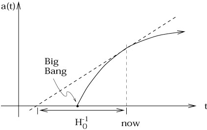
in the universe works against the expansion. The fact that
the universe can only decelerate means that it must have been
expanding even faster in the past; if we trace the evolution
backwards in time, we necessarily reach a singularity at
a = 0. Notice that if
> 0),
this means that the universe is "decelerating." This is what
we should expect, since the gravitational attraction of the matter
in the universe works against the expansion. The fact that
the universe can only decelerate means that it must have been
expanding even faster in the past; if we trace the evolution
backwards in time, we necessarily reach a singularity at
a = 0. Notice that if ![]() were exactly zero, a(t)
would be a straight line, and the age of the universe would be
H0-1. Since
were exactly zero, a(t)
would be a straight line, and the age of the universe would be
H0-1. Since ![]() is actually negative, the universe
must be somewhat younger than that.
is actually negative, the universe
must be somewhat younger than that.
|
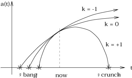
This singularity at a = 0 is the Big Bang.
It represents the creation of the universe from a singular state,
not explosion of matter into a pre-existing spacetime. It might be
hoped that the perfect symmetry of our FRW universes was responsible
for this singularity, but in fact it's not true; the singularity
theorems predict that any universe with ![]() > 0 and p
> 0 and p ![]() 0 must
have begun at a singularity. Of course
the energy density becomes arbitrarily high as
a
0 must
have begun at a singularity. Of course
the energy density becomes arbitrarily high as
a ![]() 0,
and we don't expect classical general relativity to be an
accurate description of nature in this regime; hopefully a
consistent theory of quantum gravity will be able to fix things up.
0,
and we don't expect classical general relativity to be an
accurate description of nature in this regime; hopefully a
consistent theory of quantum gravity will be able to fix things up.
The future evolution is different for different values of k.
For the open and flat cases, k ![]() 0, (8.36) implies
0, (8.36) implies
| (8.42) |
The right hand side is strictly positive (since we are
assuming ![]() > 0), so
> 0), so ![]() never passes through zero. Since
we know that today
never passes through zero. Since
we know that today ![]() > 0, it must be positive for all time.
Thus, the open and flat universes expand forever - they are
temporally as well as spatially open. (Please keep
in mind what assumptions go into this - namely, that there
is a nonzero positive energy density. Negative energy density
universes do not have to expand forever, even if they are "open".)
> 0, it must be positive for all time.
Thus, the open and flat universes expand forever - they are
temporally as well as spatially open. (Please keep
in mind what assumptions go into this - namely, that there
is a nonzero positive energy density. Negative energy density
universes do not have to expand forever, even if they are "open".)
How fast do these universes keep expanding? Consider the
quantity ![]() a3 (which is constant in matter-dominated
universes). By the conservation of energy equation (8.20) we have
a3 (which is constant in matter-dominated
universes). By the conservation of energy equation (8.20) we have
| (8.43) |
The right hand side is either zero or negative; therefore

| (8.44) |
This implies in turn that ![]() a2 must go to zero in an
ever-expanding universe, where
a
a2 must go to zero in an
ever-expanding universe, where
a ![]()
![]() . Thus (8.42)
tells us that
. Thus (8.42)
tells us that

| (8.45) |
(Remember that this is true for k ![]() 0.) Thus, for k = - 1
the expansion approaches the limiting value
0.) Thus, for k = - 1
the expansion approaches the limiting value
![]()
![]() 1,
while for k = 0 the universe keeps expanding, but more and more
slowly.
1,
while for k = 0 the universe keeps expanding, but more and more
slowly.
For the closed universes (k = + 1), (8.36) becomes
| (8.46) |
The argument that
![]() a2
a2 ![]() 0 as
a
0 as
a ![]()
![]() still applies; but in that case (8.46) would become negative, which
can't happen. Therefore the universe does not expand indefinitely;
a possesses an upper bound
amax. As a approaches
amax, (8.35) implies
still applies; but in that case (8.46) would become negative, which
can't happen. Therefore the universe does not expand indefinitely;
a possesses an upper bound
amax. As a approaches
amax, (8.35) implies
| (8.47) |
Thus ![]() is finite and negative at this point, so a
reaches
amax and starts decreasing, whereupon (since
is finite and negative at this point, so a
reaches
amax and starts decreasing, whereupon (since
![]() < 0)
it will inevitably continue to contract to zero - the Big Crunch.
Thus, the closed universes (again, under our assumptions of
positive
< 0)
it will inevitably continue to contract to zero - the Big Crunch.
Thus, the closed universes (again, under our assumptions of
positive ![]() and nonnegative p) are closed in time as well
as space.
and nonnegative p) are closed in time as well
as space.
|
We will now list some of the exact solutions corresponding to
only one type of energy density.
For dust-only universes (p = 0), it is convenient to define
a development angle ![]() (t), rather than using t as
a parameter directly. The solutions are then, for open
universes,
(t), rather than using t as
a parameter directly. The solutions are then, for open
universes,
| (8.48) |
for flat universes,
| (8.49) |
and for closed universes,
| (8.50) |
where we have defined
| (8.51) |
For universes filled with nothing but radiation,
p = ![]()
![]() ,
we have once again open universes,
,
we have once again open universes,
| (8.52) |
flat universes,
| (8.53) |
and closed universes,
| (8.54) |
where this time we defined
| (8.55) |
You can check for yourselves that these exact solutions have the properties we argued would hold in general.
For universes which are empty save for the cosmological constant,
either ![]() or p will be negative, in violation of the
assumptions we used earlier to derive the general behavior of
a(t). In this case the connection between open/closed and
expands forever/recollapses is lost. We begin by considering
or p will be negative, in violation of the
assumptions we used earlier to derive the general behavior of
a(t). In this case the connection between open/closed and
expands forever/recollapses is lost. We begin by considering
![]() < 0. In this case
< 0. In this case ![]() is negative, and from (8.41) this can only happen if k = - 1.
The solution in this case is
is negative, and from (8.41) this can only happen if k = - 1.
The solution in this case is
| (8.56) |
There is also an open (k = - 1) solution for ![]() > 0, given by
> 0, given by
| (8.57) |
A flat vacuum-dominated universe must have ![]() > 0, and the
solution is
> 0, and the
solution is
| (8.58) |
while the closed universe must also have ![]() > 0, and satisfies
> 0, and satisfies
| (8.59) |
These solutions are a little misleading. In fact the three
solutions for ![]() > 0 - (8.57), (8.58), and (8.59) -
all represent the same spacetime, just in different coordinates.
This spacetime, known as de Sitter space, is actually
maximally symmetric as a spacetime. (See Hawking and Ellis for
details.) The
> 0 - (8.57), (8.58), and (8.59) -
all represent the same spacetime, just in different coordinates.
This spacetime, known as de Sitter space, is actually
maximally symmetric as a spacetime. (See Hawking and Ellis for
details.) The ![]() < 0 solution (8.56) is
also maximally symmetric, and is known as anti-de Sitter space.
< 0 solution (8.56) is
also maximally symmetric, and is known as anti-de Sitter space.
It is clear that we would like to observationally determine a
number of quantities to decide which of the FRW models
corresponds to our universe. Obviously we would like to determine
H0, since that is related to the age of the universe.
(For a
purely matter-dominated, k = 0 universe, (8.49) implies that the
age is 2 / (3H0). Other possibilities would predict
similar relations.) We would also like to know ![]() , which determines
k through (8.41). Given the definition (8.39) of
, which determines
k through (8.41). Given the definition (8.39) of ![]() ,
this means we want to know both H0 and
,
this means we want to know both H0 and ![]() . Unfortunately
both quantities are hard to measure accurately, especially
. Unfortunately
both quantities are hard to measure accurately, especially ![]() .
But notice that the deceleration parameter q can be related
to
.
But notice that the deceleration parameter q can be related
to ![]() using (8.35):
using (8.35):
| (8.60) |
Therefore, if we think we know what w is (i.e., what kind
of stuff the universe is made of), we can determine ![]() by
measuring q. (Unfortunately we are not completely confident that
we know w, and q is itself hard to measure. But people are
trying.)
by
measuring q. (Unfortunately we are not completely confident that
we know w, and q is itself hard to measure. But people are
trying.)
To understand how these quantities might conceivably be measured,
let's consider geodesic motion in an FRW universe. There are a
number of spacelike Killing vectors, but no timelike Killing vector
to give us a notion of conserved energy. There is, however, a
Killing tensor. If
U![]() = (1, 0, 0, 0) is the four-velocity of
comoving observers, then the tensor
= (1, 0, 0, 0) is the four-velocity of
comoving observers, then the tensor
| (8.61) |
satisfies
![]() K
K![]()
![]() ) = 0 (as you can check), and is
therefore a Killing tensor. This means that if a particle has
four-velocity
V
) = 0 (as you can check), and is
therefore a Killing tensor. This means that if a particle has
four-velocity
V![]() = dx
= dx![]() /d
/d![]() , the quantity
, the quantity

| (8.62) |
will be a constant along geodesics. Let's think about this, first
for massive particles. Then we will have
V![]() V
V![]() = - 1, or
= - 1, or
| (8.63) |
where
|![]() |2 =
gijViVj. So
(8.61) implies
|2 =
gijViVj. So
(8.61) implies

| (8.64) |
The particle therefore "slows down" with respect to the comoving coordinates as the universe expands. In fact this is an actual slowing down, in the sense that a gas of particles with initially high relative velocities will cool down as the universe expands.
A similar thing happens to null geodesics. In this case
V![]() V
V![]() = 0, and (8.62) implies
= 0, and (8.62) implies

| (8.65) |
But the frequency of the photon as measured by a comoving
observer is
![]() = - U
= - U![]() V
V![]() . The frequency of the photon
emitted with frequency
. The frequency of the photon
emitted with frequency ![]() will therefore be observed with
a lower frequency
will therefore be observed with
a lower frequency ![]() as the universe expands:
as the universe expands:

| (8.66) |
Cosmologists like to speak of this in terms of the redshift z between the two events, defined by the fractional change in wavelength:

| (8.67) |
Notice that this redshift is not the same as the conventional Doppler effect; it is the expansion of space, not the relative velocities of the observer and emitter, which leads to the redshift.
The redshift is something we can measure; we know the rest-frame wavelengths of various spectral lines in the radiation from distant galaxies, so we can tell how much their wavelengths have changed along the path from time t1 when they were emitted to time t0 when they were observed. We therefore know the ratio of the scale factors at these two times. But we don't know the times themselves; the photons are not clever enough to tell us how much coordinate time has elapsed on their journey. We have to work harder to extract this information.
Roughly speaking, since a photon moves at the speed of light its travel time should simply be its distance. But what is the "distance" of a far away galaxy in an expanding universe? The comoving distance is not especially useful, since it is not measurable, and furthermore because the galaxies need not be comoving in general. Instead we can define the luminosity distance as

| (8.68) |
where L is the absolute luminosity of the source and F is
the flux measured by the observer (the energy per unit time per
unit area of some detector). The definition comes from the
fact that in flat space, for a source at distance d the flux
over the luminosity is just one over the area of a sphere centered
around the source,
F/L = 1/A(d )= 1/4![]() d2. In an FRW universe,
however, the flux will be diluted. Conservation of photons
tells us that the total number of photons emitted by
the source will eventually pass through a sphere at comoving
distance r from the emitter. Such a sphere is at a physical
distance d = a0r, where
a0 is the scale factor when the photons
are observed. But the flux is diluted by two additional effects:
the individual photons redshift by a factor (1 + z), and the photons
hit the sphere less frequently, since two photons emitted a time
d2. In an FRW universe,
however, the flux will be diluted. Conservation of photons
tells us that the total number of photons emitted by
the source will eventually pass through a sphere at comoving
distance r from the emitter. Such a sphere is at a physical
distance d = a0r, where
a0 is the scale factor when the photons
are observed. But the flux is diluted by two additional effects:
the individual photons redshift by a factor (1 + z), and the photons
hit the sphere less frequently, since two photons emitted a time
![]() t apart will be measured at a time
(1 + z)
t apart will be measured at a time
(1 + z)![]() t apart.
Therefore we will have
t apart.
Therefore we will have
| (8.69) |
or
| (8.70) |
The luminosity distance dL is something we might hope to measure, since there are some astrophysical sources whose absolute luminosities are known ("standard candles"). But r is not observable, so we have to remove that from our equation. On a null geodesic (chosen to be radial for convenience) we have
| (8.71) |
or
| (8.72) |
For galaxies not too far away, we can expand the scale factor in a Taylor series about its present value:
| (8.73) |
We can then expand both sides of (8.72) to find
| (8.74) |
Now remembering (8.67), the expansion (8.73) is the same as
| (8.75) |
For small H0(t1 - t0) this can be inverted to yield
| (8.76) |
Substituting this back again into (8.74) gives
| (8.77) |
Finally, using this in (8.70) yields Hubble's Law:
| (8.78) |
Therefore, measurement of the luminosity distances and redshifts of a sufficient number of galaxies allows us to determine H0 and q0, and therefore takes us a long way to deciding what kind of FRW universe we live in. The observations themselves are extremely difficult, and the values of these parameters in the real world are still hotly contested. Over the next decade or so a variety of new strategies and more precise application of old strategies could very well answer these questions once and for all.