


When we first derived Einstein's equations, we checked that we were on the right track by considering the Newtonian limit. This amounted to the requirements that the gravitational field be weak, that it be static (no time derivatives), and that test particles be moving slowly. In this section we will consider a less restrictive situation, in which the field is still weak but it can vary with time, and there are no restrictions on the motion of test particles. This will allow us to discuss phenomena which are absent or ambiguous in the Newtonian theory, such as gravitational radiation (where the field varies with time) and the deflection of light (which involves fast-moving particles).
The weakness of the gravitational field is once again expressed as our ability to decompose the metric into the flat Minkowski metric plus a small perturbation,
| (6.1) |
We will restrict ourselves to coordinates in which
![]() takes its canonical form,
takes its canonical form,
![]() = diag(- 1, + 1, + 1, + 1). The
assumption that
h
= diag(- 1, + 1, + 1, + 1). The
assumption that
h![]()
![]() is small allows us to ignore anything that
is higher than first order in this quantity, from which we immediately
obtain
is small allows us to ignore anything that
is higher than first order in this quantity, from which we immediately
obtain
| (6.2) |
where
h![]()
![]() =
= ![]()
![]() h
h![]()
![]() . As before,
we can raise and lower indices using
. As before,
we can raise and lower indices using
![]() and
and
![]() , since
the corrections would be of higher order in the perturbation.
In fact, we can think of the linearized version of general relativity
(where effects of higher than first order in
h
, since
the corrections would be of higher order in the perturbation.
In fact, we can think of the linearized version of general relativity
(where effects of higher than first order in
h![]()
![]() are neglected)
as describing a theory of a symmetric tensor field
h
are neglected)
as describing a theory of a symmetric tensor field
h![]()
![]() propagating on a flat background spacetime. This theory is Lorentz
invariant in the sense of special relativity; under a Lorentz
transformation
x
propagating on a flat background spacetime. This theory is Lorentz
invariant in the sense of special relativity; under a Lorentz
transformation
x![]() =
= ![]()
![]() x
x![]() , the
flat metric
, the
flat metric
![]() is invariant, while the perturbation transforms
as
is invariant, while the perturbation transforms
as
| (6.3) |
(Note that we could have considered small perturbations about some
other background spacetime besides Minkowski space. In that case
the metric would have been written
g![]()
![]() = g
= g![]()
![]() (0) + h
(0) + h![]()
![]() , and
we would have derived a theory of a symmetric tensor propagating on
the curved space with metric
g
, and
we would have derived a theory of a symmetric tensor propagating on
the curved space with metric
g![]()
![]() (0). Such an approach is
necessary, for example, in cosmology.)
(0). Such an approach is
necessary, for example, in cosmology.)
We want to find the equation of motion obeyed by the perturbations
h![]()
![]() , which come by examining Einstein's
equations to first order.
We begin with the Christoffel symbols, which are given by
, which come by examining Einstein's
equations to first order.
We begin with the Christoffel symbols, which are given by
| (6.4) |
Since the connection coefficients are first order quantities, the
only contribution to the Riemann tensor will come from the derivatives
of the ![]() 's, not the
's, not the ![]() terms. Lowering an index for
convenience, we obtain
terms. Lowering an index for
convenience, we obtain
| (6.5) |
The Ricci tensor comes from contracting over ![]() and
and ![]() ,
giving
,
giving
| (6.6) |
which is manifestly symmetric in ![]() and
and ![]() . In this expression
we have defined the trace of the perturbation as
h =
. In this expression
we have defined the trace of the perturbation as
h = ![]() h
h![]()
![]() = h
= h![]()
![]() , and the D'Alembertian is simply the
one from flat space,
, and the D'Alembertian is simply the
one from flat space,
![]() = -
= - ![]() +
+ ![]() +
+ ![]() +
+ ![]() . Contracting again to
obtain the Ricci scalar yields
. Contracting again to
obtain the Ricci scalar yields
| (6.7) |
Putting it all together we obtain the Einstein tensor:
| (6.8) |
Consistent with our interpretation of the linearized theory as
one describing a symmetric tensor on a flat background, the linearized
Einstein tensor (6.8) can be derived by varying the following
Lagrangian with respect to
h![]()
![]() :
:

| (6.9) |
I will spare you the details.
The linearized field equation is of course
G![]()
![]() = 8
= 8![]() GT
GT![]()
![]() ,
where
G
,
where
G![]()
![]() is given by (6.8) and
T
is given by (6.8) and
T![]()
![]() is the energy-momentum
tensor, calculated to zeroth order in
h
is the energy-momentum
tensor, calculated to zeroth order in
h![]()
![]() . We do not include
higher-order corrections to the energy-momentum tensor because the
amount of energy and momentum must itself be small for the weak-field
limit to apply. In other words, the lowest nonvanishing order in
T
. We do not include
higher-order corrections to the energy-momentum tensor because the
amount of energy and momentum must itself be small for the weak-field
limit to apply. In other words, the lowest nonvanishing order in
T![]()
![]() is automatically of the same order of
magnitude as the
perturbation. Notice that the conservation law to lowest order is
simply
is automatically of the same order of
magnitude as the
perturbation. Notice that the conservation law to lowest order is
simply
![]() T
T![]()
![]() = 0. We will most often be concerned
with the vacuum equations, which as usual are just
R
= 0. We will most often be concerned
with the vacuum equations, which as usual are just
R![]()
![]() = 0, where
R
= 0, where
R![]()
![]() is given by (6.6).
is given by (6.6).
With the linearized field equations in hand, we are almost prepared
to set about solving them. First, however, we should deal with the
thorny issue of gauge invariance. This issue arises because the
demand that
g![]()
![]() =
= ![]() + h
+ h![]()
![]() does not completely specify the
coordinate system on spacetime; there may be other coordinate systems
in which the metric can still be written as the Minkowski metric
plus a small perturbation, but the perturbation will be different.
Thus, the decomposition of the metric into a flat background plus a
perturbation is not unique.
does not completely specify the
coordinate system on spacetime; there may be other coordinate systems
in which the metric can still be written as the Minkowski metric
plus a small perturbation, but the perturbation will be different.
Thus, the decomposition of the metric into a flat background plus a
perturbation is not unique.
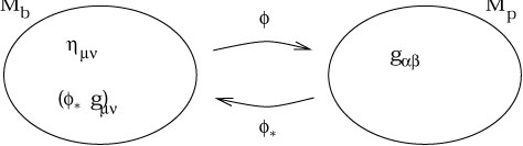
We can think about this from a highbrow point of view. The notion
that the linearized theory can be thought of as one governing the
behavior of tensor fields on a flat background can be formalized in
terms of a "background spacetime" Mb, a "physical
spacetime" Mp, and a diffeomorphism
![]() : Mb
: Mb ![]() Mp. As manifolds
Mb and Mp are "the same" (since they
are diffeomorphic), but
we imagine that they possess some different tensor fields;
on Mb we have defined the flat Minkowski metric
Mp. As manifolds
Mb and Mp are "the same" (since they
are diffeomorphic), but
we imagine that they possess some different tensor fields;
on Mb we have defined the flat Minkowski metric
![]() , while
on Mp we have some metric
g
, while
on Mp we have some metric
g![]()
![]() which obeys Einstein's
equations. (We imagine that Mb is equipped with
coordinates
x
which obeys Einstein's
equations. (We imagine that Mb is equipped with
coordinates
x![]() and Mp is equipped
with coordinates y
and Mp is equipped
with coordinates y![]() , although
these will not play a prominent role.)
The diffeomorphism
, although
these will not play a prominent role.)
The diffeomorphism ![]() allows us to move tensors back
and forth between the background and physical spacetimes. Since we
would like to construct our linearized theory as one taking place
on the flat background spacetime, we are interested in the pullback
(
allows us to move tensors back
and forth between the background and physical spacetimes. Since we
would like to construct our linearized theory as one taking place
on the flat background spacetime, we are interested in the pullback
(![]() g)
g)![]()
![]() of the physical metric. We can define
the perturbation
as the difference between the pulled-back physical metric and the
flat one:
of the physical metric. We can define
the perturbation
as the difference between the pulled-back physical metric and the
flat one:
| (6.10) |
From this definition, there is no reason for the components of
h![]()
![]() to be small; however, if the gravitational fields on
Mp are weak, then for some diffeomorphisms
to be small; however, if the gravitational fields on
Mp are weak, then for some diffeomorphisms ![]() we will have | h
we will have | h![]()
![]() | < < 1.
We therefore limit our attention only to those diffeomorphisms for which
this is true. Then the fact that
g
| < < 1.
We therefore limit our attention only to those diffeomorphisms for which
this is true. Then the fact that
g![]()
![]() obeys Einstein's
equations on the physical spacetime means that
h
obeys Einstein's
equations on the physical spacetime means that
h![]()
![]() will obey
the linearized equations on the background spacetime (since
will obey
the linearized equations on the background spacetime (since ![]() ,
as a diffeomorphism, can be used to pull back Einstein's equations
themselves).
,
as a diffeomorphism, can be used to pull back Einstein's equations
themselves).
|
In this language, the issue of gauge invariance is simply the fact that
there are a large number of permissible diffeomorphisms between
Mb
and Mp (where "permissible" means that the
perturbation is small). Consider a vector field
![]() (x) on the background spacetime.
This vector field generates a one-parameter family of diffeomorphisms
(x) on the background spacetime.
This vector field generates a one-parameter family of diffeomorphisms
![]() : Mb
: Mb ![]() Mb. For
Mb. For ![]() sufficiently small,
if
sufficiently small,
if ![]() is a diffeomorphism for which the perturbation defined
by (6.10) is small than so will
(
is a diffeomorphism for which the perturbation defined
by (6.10) is small than so will
(![]() o
o![]() ) be, although
the perturbation will have a different value.
) be, although
the perturbation will have a different value.

|
Specifically, we can
define a family of perturbations parameterized by ![]() :
:
| (6.11) |
The second equality is based on the fact that the pullback under a composition is given by the composition of the pullbacks in the opposite order, which follows from the fact that the pullback itself moves things in the opposite direction from the original map. Plugging in the relation (6.10), we find
| (6.12) |
(since the pullback of the sum of two tensors is the sum of the
pullbacks). Now we use our assumption that ![]() is small; in
this case
is small; in
this case
![]() (h
(h![]()
![]() ) will be equal to
h
) will be equal to
h![]()
![]() to
lowest order, while the other two terms give us a Lie derivative:
to
lowest order, while the other two terms give us a Lie derivative:
| (6.13) |
The last equality follows from our previous computation of the Lie derivative of the metric, (5.33), plus the fact that covariant derivatives are simply partial derivatives to lowest order.
The infinitesimal diffeomorphisms
![]() provide a
different representation of the same physical situation, while
maintaining our requirement that the perturbation be small. Therefore,
the result (6.12) tells us what kind of metric perturbations denote
physically equivalent spacetimes - those related to each other by
2
provide a
different representation of the same physical situation, while
maintaining our requirement that the perturbation be small. Therefore,
the result (6.12) tells us what kind of metric perturbations denote
physically equivalent spacetimes - those related to each other by
2![]()
![]()
![]() , for some vector
, for some vector ![]() .
The invariance of our theory under such transformations is analogous
to traditional gauge invariance of electromagnetism under
A
.
The invariance of our theory under such transformations is analogous
to traditional gauge invariance of electromagnetism under
A![]()
![]() A
A![]() +
+ ![]()
![]() . (The analogy is
different from the previous analogy we drew with electromagnetism,
relating local Lorentz transformations in the orthonormal-frame
formalism to changes of basis in an internal vector bundle.) In
electromagnetism the invariance comes about because the field
strength
F
. (The analogy is
different from the previous analogy we drew with electromagnetism,
relating local Lorentz transformations in the orthonormal-frame
formalism to changes of basis in an internal vector bundle.) In
electromagnetism the invariance comes about because the field
strength
F![]()
![]() =
= ![]() A
A![]() -
- ![]() A
A![]() is left unchanged by
gauge transformations; similarly, we find that the transformation (6.13)
changes the linearized Riemann tensor by
is left unchanged by
gauge transformations; similarly, we find that the transformation (6.13)
changes the linearized Riemann tensor by
| (6.14) |
Our abstract derivation of the appropriate gauge transformation for the metric perturbation is verified by the fact that it leaves the curvature (and hence the physical spacetime) unchanged.
Gauge invariance can also be understood from the slightly more
lowbrow but considerably more direct route of infinitesimal coordinate
transformations. Our diffeomorphism
![]() can be thought
of as changing coordinates from x
can be thought
of as changing coordinates from x![]() to
x
to
x![]() -
- ![]()
![]() .
(The minus sign, which is unconventional, comes from the fact that the
"new" metric is pulled back from a small distance forward along the
integral curves, which is equivalent to replacing the coordinates by
those a small distance backward along the curves.) Following through
the usual rules for transforming tensors under coordinate transformations,
you can derive precisely (6.13) - although you have to cheat somewhat
by equating components of tensors in two different coordinate systems.
See Schutz or Weinberg for an example.
.
(The minus sign, which is unconventional, comes from the fact that the
"new" metric is pulled back from a small distance forward along the
integral curves, which is equivalent to replacing the coordinates by
those a small distance backward along the curves.) Following through
the usual rules for transforming tensors under coordinate transformations,
you can derive precisely (6.13) - although you have to cheat somewhat
by equating components of tensors in two different coordinate systems.
See Schutz or Weinberg for an example.
When faced with a system that is invariant under some kind of gauge
transformations, our first instinct is to fix a gauge. We have
already discussed the harmonic coordinate system, and will return to
it now in the context of the weak field limit. Recall that this gauge
was specified by
![]() x
x![]() = 0, which we showed was equivalent to
= 0, which we showed was equivalent to

| (6.15) |
In the weak field limit this becomes
| (6.16) |
or
| (6.17) |
This condition is also known as Lorentz gauge (or Einstein gauge or Hilbert gauge or de Donder gauge or Fock gauge). As before, we still have some gauge freedom remaining, since we can change our coordinates by (infinitesimal) harmonic functions.
In this gauge, the linearized Einstein equations
G![]()
![]() = 8
= 8![]() GT
GT![]()
![]() simplify somewhat, to
simplify somewhat, to
| (6.18) |
while the vacuum equations
R![]()
![]() = 0 take on the elegant form
= 0 take on the elegant form

| (6.19) |
which is simply the conventional relativistic wave equation. Together, (6.19) and (6.17) determine the evolution of a disturbance in the gravitational field in vacuum in the harmonic gauge.
It is often convenient to work with a slightly different description
of the metric perturbation. We define the "trace-reversed" perturbation
![]() by
by
| (6.20) |
The name makes sense, since
![]()
![]() = - h
= - h![]()
![]() . (The
Einstein tensor is simply the trace-reversed Ricci tensor.) In
terms of
. (The
Einstein tensor is simply the trace-reversed Ricci tensor.) In
terms of
![]() the harmonic gauge condition becomes
the harmonic gauge condition becomes

| (6.21) |
The full field equations are
| (6.22) |
from which it follows immediately that the vacuum equations are

| (6.23) |
From (6.22) and our previous exploration of the Newtonian limit, it is straightforward to derive the weak-field metric for a stationary spherical source such as a planet or star. Recall that previously we found that Einstein's equations predicted that h00 obeyed the Poisson equation (4.51) in the weak-field limit, which implied

| (6.24) |
where ![]() is the conventional Newtonian potential,
is the conventional Newtonian potential,
![]() = - GM/r.
Let us now assume that the energy-momentum tensor of our source is
dominated by its rest energy density
= - GM/r.
Let us now assume that the energy-momentum tensor of our source is
dominated by its rest energy density
![]() = T00. (Such an
assumption is not generally necessary in the weak-field limit, but
will certainly hold for a planet or star, which is what we would
like to consider for the moment.) Then the other components of
T
= T00. (Such an
assumption is not generally necessary in the weak-field limit, but
will certainly hold for a planet or star, which is what we would
like to consider for the moment.) Then the other components of
T![]()
![]() will be much smaller than
T00, and from (6.22) the same must hold for
will be much smaller than
T00, and from (6.22) the same must hold for
![]() .
If
.
If
![]() is much larger than
is much larger than
![]() , we will have
, we will have
| (6.25) |
and then from (6.20) we immediately obtain
| (6.26) |
The other components of
![]() are negligible, from which
we can derive
are negligible, from which
we can derive
| (6.27) |
and
| (6.28) |
The metric for a star or planet in the weak-field limit is therefore

| (6.29) |
A somewhat less simplistic application of the weak-field limit
is to gravitational radiation. Those of you familiar with the
analogous problem in electromagnetism will notice that the
procedure is almost precisely the same. We begin by considering the
linearized equations in vacuum (6.23). Since the flat-space
D'Alembertian has the form
![]() = -
= - ![]() +
+ ![]() , the field
equation is in the form of a wave equation for
, the field
equation is in the form of a wave equation for
![]() . As all
good physicists know, the thing to do when faced with such an equation
is to write down complex-valued solutions, and then take the real
part at the very end of the day. So we recognize that a particularly
useful set of solutions to this wave equation are the plane waves, given
by
. As all
good physicists know, the thing to do when faced with such an equation
is to write down complex-valued solutions, and then take the real
part at the very end of the day. So we recognize that a particularly
useful set of solutions to this wave equation are the plane waves, given
by
| (6.30) |
where
C![]()
![]() is a constant, symmetric, (0, 2)
tensor,
and k
is a constant, symmetric, (0, 2)
tensor,
and k![]() is a constant vector known as the wave vector.
To check that it is a solution, we plug in:
is a constant vector known as the wave vector.
To check that it is a solution, we plug in:
| (6.31) |
Since (for an interesting solution) not all of the components of
h![]()
![]() will be zero everywhere, we must have
will be zero everywhere, we must have

| (6.32) |
The plane wave (6.30) is therefore a solution to the linearized
equations if the wavevector is null; this is loosely translated into
the statement that gravitational waves propagate at the speed of light.
The timelike component of the wave vector is often referred to as
the frequency of the wave, and we write
k![]() = (
= (![]() , k1, k2,
k3). (More generally, an observer moving with
four-velocity
U
, k1, k2,
k3). (More generally, an observer moving with
four-velocity
U![]() would observe the wave to have a frequency
would observe the wave to have a frequency
![]() = - k
= - k![]() U
U![]() .)
Then the condition that the wave vector be null becomes
.)
Then the condition that the wave vector be null becomes

| (6.33) |
Of course our wave is far from the most general solution; any (possibly infinite) number of distinct plane waves can be added together and will still solve the linear equation (6.23). Indeed, any solution can be written as such a superposition.
There are a number of free parameters to specify the wave: ten numbers
for the coefficients
C![]()
![]() and three for the null vector
k
and three for the null vector
k![]() .
Much of these are the result of coordinate freedom and gauge freedom,
which we now set about eliminating. We begin by imposing the
harmonic gauge condition, (6.21). This implies that
.
Much of these are the result of coordinate freedom and gauge freedom,
which we now set about eliminating. We begin by imposing the
harmonic gauge condition, (6.21). This implies that
| (6.34) |
which is only true if

| (6.35) |
We say that the wave vector is orthogonal to
C![]()
![]() . These are four
equations, which reduce the number of independent components of
C
. These are four
equations, which reduce the number of independent components of
C![]()
![]() from ten to six.
from ten to six.
Although we have now imposed the harmonic gauge condition, there is still some coordinate freedom left. Remember that any coordinate transformation of the form

| (6.36) |
will leave the harmonic coordinate condition

| (6.37) |
satisfied as long as we have

| (6.38) |
Of course, (6.38) is itself a wave equation for ![]() ; once
we choose a solution, we will have used up all of our gauge freedom.
Let's choose the following solution:
; once
we choose a solution, we will have used up all of our gauge freedom.
Let's choose the following solution:

| (6.39) |
where k![]() is the wave vector for our
gravitational wave and the B
is the wave vector for our
gravitational wave and the B![]() are constant coefficients.
are constant coefficients.
We now claim that this
remaining freedom allows us to convert from whatever coefficients
C(old)![]()
![]() that characterize our gravitational
wave to a new set
C(new)
that characterize our gravitational
wave to a new set
C(new)![]()
![]() , such that
, such that

| (6.40) |
and

| (6.41) |
(Actually this last condition is both a choice of gauge and a
choice of Lorentz frame. The choice of gauge sets
U![]() C(new)
C(new)![]()
![]() = 0 for some constant timelike vector
U
= 0 for some constant timelike vector
U![]() ,
while the choice of frame makes U
,
while the choice of frame makes U![]() point along the time axis.)
Let's see how this is possible by solving explicitly for the necessary
coefficients B
point along the time axis.)
Let's see how this is possible by solving explicitly for the necessary
coefficients B![]() . Under the transformation (6.36),
the resulting change in our metric perturbation can be written
. Under the transformation (6.36),
the resulting change in our metric perturbation can be written
| (6.42) |
which induces a change in the trace-reversed perturbation,
| (6.43) |
Using the specific forms (6.30) for the solution and (6.39) for the transformation, we obtain

| (6.44) |
Imposing (6.40) therefore means
| (6.45) |
or
| (6.46) |
Then we can impose (6.41), first for ![]() = 0:
= 0:
| (6.47) |
or
| (6.48) |
Then impose (6.41) for ![]() = j:
= j:
| (6.49) |
or
| (6.50) |
To check that these choices are mutually consistent, we should plug
(6.48) and (6.50) back into (6.40), which I will leave to you.
Let us assume that we have performed this transformation, and refer
to the new components
C![]()
![]() (new) simply as
C
(new) simply as
C![]()
![]() .
.
Thus, we began with the ten independent numbers in the symmetric
matrix
C![]()
![]() . Choosing harmonic gauge implied the
four conditions
(6.35), which brought the number of independent components down to
six. Using our remaining gauge freedom led to the one condition (6.40)
and the four conditions (6.41); but when
. Choosing harmonic gauge implied the
four conditions
(6.35), which brought the number of independent components down to
six. Using our remaining gauge freedom led to the one condition (6.40)
and the four conditions (6.41); but when ![]() = 0 (6.41) implies
(6.35), so we have a total of four additional constraints, which
brings us to two independent components. We've used up all of our
possible freedom, so these two numbers represent the physical
information characterizing our plane wave in this gauge. This can
be seen more explicitly by choosing our spatial coordinates such
that the wave is travelling in the x3 direction; that is,
= 0 (6.41) implies
(6.35), so we have a total of four additional constraints, which
brings us to two independent components. We've used up all of our
possible freedom, so these two numbers represent the physical
information characterizing our plane wave in this gauge. This can
be seen more explicitly by choosing our spatial coordinates such
that the wave is travelling in the x3 direction; that is,
| (6.51) |
where we know that
k3 = ![]() because the wave vector is null.
In this case,
k
because the wave vector is null.
In this case,
k![]() C
C![]()
![]() = 0 and
C0
= 0 and
C0![]() = 0 together imply
= 0 together imply

| (6.52) |
The only nonzero components of
C![]()
![]() are therefore C11,
C12, C21, and
C22. But C
are therefore C11,
C12, C21, and
C22. But C![]()
![]() is traceless and
symmetric, so in general we can write
is traceless and
symmetric, so in general we can write
| (6.53) |
Thus, for a plane wave in this gauge travelling in the x3
direction, the two components C11 and
C12 (along with the frequency ![]() ) completely characterize the wave.
) completely characterize the wave.
In using up all of our gauge freedom, we have gone to a subgauge of
the harmonic gauge known as the transverse traceless gauge
(or sometimes "radiation gauge"). The name comes from the fact
that the metric perturbation is traceless and perpendicular to the
wave vector. Of course, we have been working with the trace-reversed
perturbation
![]() rather than the perturbation
h
rather than the perturbation
h![]()
![]() itself; but since
itself; but since
![]() is traceless (because
C
is traceless (because
C![]()
![]() is), and is equal to
the trace-reverse of
h
is), and is equal to
the trace-reverse of
h![]()
![]() , in this gauge we have
, in this gauge we have

| (6.54) |
Therefore we can drop the bars over
h![]()
![]() , as long as we are in
this gauge.
, as long as we are in
this gauge.
One nice feature of the transverse traceless gauge is that if you
are given the components of a plane wave in some arbitrary gauge, you
can easily convert them into the transverse traceless components.
We first define a tensor
P![]()
![]() which acts as a projection operator:
which acts as a projection operator:
| (6.55) |
You can check that this projects vectors onto hyperplanes orthogonal
to the unit vector n![]() . Here we take
n
. Here we take
n![]() to be a spacelike unit vector,
which we choose
to lie along the direction of propagation of the wave:
to be a spacelike unit vector,
which we choose
to lie along the direction of propagation of the wave:
| (6.56) |
Then the transverse part of some perturbation
h![]()
![]() is simply
the projection P
is simply
the projection P![]()
![]() P
P![]()
![]() h
h![]()
![]() , and
the transverse traceless part is obtained by subtracting off the
trace:
, and
the transverse traceless part is obtained by subtracting off the
trace:
| (6.57) |
For details appropriate to more general cases, see the discussion in Misner, Thorne and Wheeler.
To get a feeling for the physical effects due to gravitational
waves, it is useful to consider the motion of test particles in
the presence of a wave. It is certainly insufficient to solve
for the trajectory of a single particle, since that would only
tell us about the values of the coordinates along the world line.
(In fact, for any single particle we can find transverse traceless
coordinates in which the particle appears stationary to first
order in
h![]()
![]() .)
To obtain a coordinate-independent measure of the wave's effects,
we consider the relative motion of nearby particles, as described
by the geodesic deviation equation. If we consider some nearby
particles with four-velocities described by a single vector field
U
.)
To obtain a coordinate-independent measure of the wave's effects,
we consider the relative motion of nearby particles, as described
by the geodesic deviation equation. If we consider some nearby
particles with four-velocities described by a single vector field
U![]() (x) and separation vector
S
(x) and separation vector
S![]() , we have
, we have
| (6.58) |
We would like to compute the left-hand side to first order in
h![]()
![]() . If we take our test particles to be
moving slowly
then we can express the four-velocity as a unit vector in the
time direction plus corrections of order h
. If we take our test particles to be
moving slowly
then we can express the four-velocity as a unit vector in the
time direction plus corrections of order h![]()
![]() and higher;
but we know that the Riemann tensor is already first order, so
the corrections to U
and higher;
but we know that the Riemann tensor is already first order, so
the corrections to U![]() may be ignored, and we write
may be ignored, and we write
| (6.59) |
Therefore we only need to compute
R![]() 00
00![]() , or
equivalently R
, or
equivalently R![]() 00
00![]() . From (6.5) we have
. From (6.5) we have
| (6.60) |
But
h![]() 0 = 0, so
0 = 0, so
| (6.61) |
Meanwhile, for our slowly-moving particles we have
![]() = x0 = t
to lowest order, so the geodesic deviation equation becomes
= x0 = t
to lowest order, so the geodesic deviation equation becomes
| (6.62) |
For our wave travelling in the x3 direction, this implies that only S1 and S2 will be affected - the test particles are only disturbed in directions perpendicular to the wave vector. This is of course familiar from electromagnetism, where the electric and magnetic fields in a plane wave are perpendicular to the wave vector.
Our wave is characterized by the two numbers, which for future convenience we will rename as C+ = C11 and C × = C12. Let's consider their effects separately, beginning with the case C × = 0. Then we have
| (6.63) |
and
| (6.64) |
These can be immediately solved to yield, to lowest order,
| (6.65) |
and
| (6.66) |
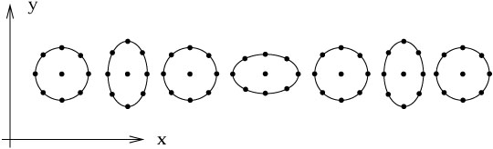
Thus, particles initially separated in the x1 direction will oscillate back and forth in the x1 direction, and likewise for those with an initial x2 separation. That is, if we start with a ring of stationary particles in the x-y plane, as the wave passes they will bounce back and forth in the shape of a "+":
|
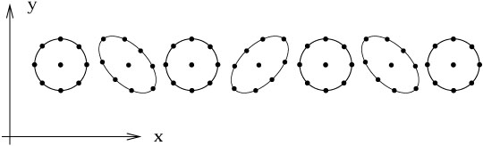
On the other hand, the equivalent analysis for the
case where C+ = 0 but
C × ![]() 0 would yield the solution
0 would yield the solution
| (6.67) |
and
| (6.68) |
In this case the circle of particles would bounce back and forth in the shape of a "×":
|
The notation C+ and C × should therefore be clear. These two quantities measure the two independent modes of linear polarization of the gravitational wave. If we liked we could consider right- and left-handed circularly polarized modes by defining
| (6.69) |
The effect of a pure CR wave would be to rotate the particles in a right-handed sense,

|
and similarly for the left-handed mode CL. (Note that the individual particles do not travel around the ring; they just move in little epicycles.)
We can relate the polarization states of classical gravitational waves
to the kinds of particles we would expect to find upon
quantization. The electromagnetic field has two independent
polarization states which are described by vectors in
the x-y plane; equivalently, a single polarization mode
is invariant under a rotation by 360° in this plane.
Upon quantization this theory yields the photon, a massless
spin-one particle. The neutrino, on the other hand, is also a
massless particle, described by a field which picks up a
minus sign under rotations by 360°; it is invariant
under rotations of 720°, and we say it has
spin-![]() . The general rule is that the spin S is
related to the angle
. The general rule is that the spin S is
related to the angle ![]() under which the polarization modes
are invariant by
S = 360°/
under which the polarization modes
are invariant by
S = 360°/![]() .
The gravitational field, whose waves
propagate at the speed of light, should lead to massless particles
in the quantum theory. Noticing that the polarization modes we
have described are invariant under rotations of 180° in
the x-y plane, we expect the associated particles
- "gravitons" - to be
spin-2. We are a long way from detecting such particles (and it
would not be a surprise if we never detected them directly), but any
respectable quantum theory of gravity should predict their existence.
.
The gravitational field, whose waves
propagate at the speed of light, should lead to massless particles
in the quantum theory. Noticing that the polarization modes we
have described are invariant under rotations of 180° in
the x-y plane, we expect the associated particles
- "gravitons" - to be
spin-2. We are a long way from detecting such particles (and it
would not be a surprise if we never detected them directly), but any
respectable quantum theory of gravity should predict their existence.
With plane-wave solutions to the linearized vacuum equations in our possession, it remains to discuss the generation of gravitational radiation by sources. For this purpose it is necessary to consider the equations coupled to matter,
| (6.70) |
The solution to such an equation can be obtained using a Green's function, in precisely the same way as the analogous problem in electromagnetism. Here we will review the outline of the method.
The Green's function
G(x![]() - y
- y![]() ) for the D'Alembertian operator
) for the D'Alembertian operator
![]() is the solution of the wave equation in the presence of a
delta-function source:
is the solution of the wave equation in the presence of a
delta-function source:
| (6.71) |
where ![]() denotes the D'Alembertian with respect to the
coordinates x
denotes the D'Alembertian with respect to the
coordinates x![]() . The usefulness of such a function
resides in the fact that
the general solution to an equation such as (6.70) can be written
. The usefulness of such a function
resides in the fact that
the general solution to an equation such as (6.70) can be written
| (6.72) |
as can be verified immediately. (Notice that no factors of
![]() are
necessary, since our background is simply flat spacetime.) The
solutions to (6.71) have of course been worked out long ago, and
they can be thought of as either "retarded" or "advanced," depending
on whether they represent waves travelling forward or backward in time.
Our interest is in the retarded Green's function, which represents the
accumulated effects of signals to the past of the point under
consideration. It is given by
are
necessary, since our background is simply flat spacetime.) The
solutions to (6.71) have of course been worked out long ago, and
they can be thought of as either "retarded" or "advanced," depending
on whether they represent waves travelling forward or backward in time.
Our interest is in the retarded Green's function, which represents the
accumulated effects of signals to the past of the point under
consideration. It is given by
| (6.73) |
Here we have used boldface to denote the spatial vectors
![]() = (x1, x2,
x3) and
= (x1, x2,
x3) and ![]() = (y1, y2,
y3), with norm
|
= (y1, y2,
y3), with norm
|![]() -
- ![]() | = [
| = [![]() (xi -
yi)(xj -
yj)]1/2. The theta function
(xi -
yi)(xj -
yj)]1/2. The theta function
![]() (x0 - y0) equals 1
when x0 > y0, and zero
otherwise.
The derivation of (6.73) would take us too far afield, but it can be
found in any standard text on electrodynamics or partial differential
equations in physics.
(x0 - y0) equals 1
when x0 > y0, and zero
otherwise.
The derivation of (6.73) would take us too far afield, but it can be
found in any standard text on electrodynamics or partial differential
equations in physics.
Upon plugging (6.73) into (6.72), we can use the delta function to perform the integral over y0, leaving us with
| (6.74) |
where t = x0. The term "retarded time" is used to refer to the quantity
| (6.75) |
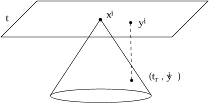
The interpretation of (6.74) should be clear: the disturbance in the
gravitational field at
(t,![]() ) is a sum of the influences from the energy
and momentum sources at the point
(tr,
) is a sum of the influences from the energy
and momentum sources at the point
(tr,![]() -
- ![]() ) on the past
light cone.
) on the past
light cone.
|
Let us take this general solution and consider the case where the
gravitational radiation is emitted by an isolated source, fairly far away,
comprised of nonrelativistic matter; these approximations will be made
more precise as we go on. First we need to set up some conventions for
Fourier transforms, which always make life easier when dealing with
oscillatory phenomena. Given a function of spacetime
![]() (t,
(t,![]() ), we
are interested in its Fourier transform (and inverse) with
respect to time alone,
), we
are interested in its Fourier transform (and inverse) with
respect to time alone,
| (6.76) |
Taking the transform of the metric perturbation, we obtain
| (6.77) |
In this sequence, the first equation is simply the definition of the Fourier transform, the second line comes from the solution (6.74), the third line is a change of variables from t to tr, and the fourth line is once again the definition of the Fourier transform.
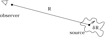
We now make the approximations that our source is isolated, far away, and
slowly moving. This means that we can consider the source to be centered
at a (spatial) distance R, with the different parts of the source at
distances
R + ![]() R such that
R such that
![]() R < < R. Since it is slowly
moving, most of the radiation emitted will be at frequencies
R < < R. Since it is slowly
moving, most of the radiation emitted will be at frequencies ![]() sufficiently low that
sufficiently low that
![]() R < <
R < < ![]() . (Essentially, light
traverses the source much faster than the components of the source itself
do.)
. (Essentially, light
traverses the source much faster than the components of the source itself
do.)
|
Under these approximations, the term
ei![]() |
|![]() -
- ![]() |/|
|/|![]() -
- ![]() | can be replaced by
ei
| can be replaced by
ei![]() R/R
and brought outside the integral. This leaves us with
R/R
and brought outside the integral. This leaves us with
| (6.78) |
In fact there is no need to compute all of the components of
![]() (
(![]() ,
,![]() ), since the harmonic gauge condition
), since the harmonic gauge condition
![]()
![]() (t,
(t,![]() ) = 0 in Fourier space implies
) = 0 in Fourier space implies

| (6.79) |
We therefore only need to concern ourselves with the spacelike
components of
![]() (
(![]() ,
,![]() ). From (6.78) we
therefore want to take the integral of the spacelike components of
). From (6.78) we
therefore want to take the integral of the spacelike components of
![]() (
(![]() ,
,![]() ). We begin by integrating by parts in
reverse:
). We begin by integrating by parts in
reverse:

| (6.80) |
The first term is a surface integral which will vanish since the
source is isolated, while the second can be related to
![]() by the Fourier-space version of
by the Fourier-space version of
![]() T
T![]()
![]() = 0:
= 0:
| (6.81) |
Thus,
| (6.82) |
The second line is justified since we know that the left hand side
is symmetric in i and j, while the third and fourth lines
are simply
repetitions of reverse integration by parts and conservation of
T![]()
![]() .
It is conventional to define the quadrupole moment tensor of the
energy density of the source,
.
It is conventional to define the quadrupole moment tensor of the
energy density of the source,
| (6.83) |
a constant tensor on each surface of constant time. In terms of the Fourier transform of the quadrupole moment, our solution takes on the compact form
| (6.84) |
or, transforming back to t,
| (6.85) |
where as before tr = t - R.
The gravitational wave produced by an isolated nonrelativistic object is therefore proportional to the second derivative of the quadrupole moment of the energy density at the point where the past light cone of the observer intersects the source. In contrast, the leading contribution to electromagnetic radiation comes from the changing dipole moment of the charge density. The difference can be traced back to the universal nature of gravitation. A changing dipole moment corresponds to motion of the center of density - charge density in the case of electromagnetism, energy density in the case of gravitation. While there is nothing to stop the center of charge of an object from oscillating, oscillation of the center of mass of an isolated system violates conservation of momentum. (You can shake a body up and down, but you and the earth shake ever so slightly in the opposite direction to compensate.) The quadrupole moment, which measures the shape of the system, is generally smaller than the dipole moment, and for this reason (as well as the weak coupling of matter to gravity) gravitational radiation is typically much weaker than electromagnetic radiation.
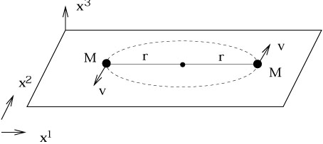
It is always educational to take a general solution and apply it to a specific case of interest. One case of genuine interest is the gravitational radiation emitted by a binary star (two stars in orbit around each other). For simplicity let us consider two stars of mass M in a circular orbit in the x1-x2 plane, at distance r from their common center of mass.
|
We will treat the motion of the stars in the Newtonian approximation, where we can discuss their orbit just as Kepler would have. Circular orbits are most easily characterized by equating the force due to gravity to the outward "centrifugal" force:

| (6.86) |
which gives us
| (6.87) |
The time it takes to complete a single orbit is simply

| (6.88) |
but more useful to us is the angular frequency of the orbit,
| (6.89) |
In terms of ![]() we can write down the explicit path of star
a,
we can write down the explicit path of star
a,
| (6.90) |
and star b,

| (6.91) |
The corresponding energy density is

| (6.92) |
The profusion of delta functions allows us to integrate this straightforwardly to obtain the quadrupole moment from (6.83):
| (6.93) |
From this in turn it is easy to get the components of the metric perturbation from (6.85):
| (6.94) |
The remaining components of
![]() could be derived from demanding
that the harmonic gauge
condition be satisfied. (We have not imposed a subsidiary gauge
condition, so we are still free to do so.)
could be derived from demanding
that the harmonic gauge
condition be satisfied. (We have not imposed a subsidiary gauge
condition, so we are still free to do so.)
It is natural at this point to talk about the energy emitted
via gravitational radiation. Such a discussion, however, is
immediately beset by problems, both technical and philosophical.
As we have mentioned before, there is no true local measure of
the energy in the gravitational field. Of course, in the weak
field limit, where we think of gravitation as being described
by a symmetric tensor propagating on a fixed background metric,
we might hope to derive an energy-momentum tensor for the
fluctuations
h![]()
![]() , just as we would for electromagnetism or
any other field theory. To some extent this is possible, but
there are still difficulties. As a result of these difficulties
there are a number of different proposals in the literature for
what we should use as the energy-momentum tensor for gravitation
in the weak field limit; all of them are different, but for
the most part they give the same answers for physically
well-posed questions such as the rate of energy emitted by a
binary system.
, just as we would for electromagnetism or
any other field theory. To some extent this is possible, but
there are still difficulties. As a result of these difficulties
there are a number of different proposals in the literature for
what we should use as the energy-momentum tensor for gravitation
in the weak field limit; all of them are different, but for
the most part they give the same answers for physically
well-posed questions such as the rate of energy emitted by a
binary system.
At a technical level, the difficulties begin to arise when we
consider what form the energy-momentum tensor should take.
We have previously mentioned the energy-momentum tensors for
electromagnetism and scalar field theory, and they both
shared an important feature - they were quadratic in the
relevant fields. By hypothesis our approach to the weak field
limit has been to only keep terms which are linear in the
metric perturbation. Hence, in order to keep track of the
energy carried by the gravitational waves, we will have to
extend our calculations to at least second order in
h![]()
![]() .
In fact we have been cheating slightly all along. In
discussing the effects of gravitational waves on test particles,
and the generation of waves by a binary system, we have been
using the fact that test particles move along geodesics. But
as we know, this is derived from the covariant conservation of
energy-momentum,
.
In fact we have been cheating slightly all along. In
discussing the effects of gravitational waves on test particles,
and the generation of waves by a binary system, we have been
using the fact that test particles move along geodesics. But
as we know, this is derived from the covariant conservation of
energy-momentum,
![]() T
T![]()
![]() = 0. In the order to which
we have been working, however, we actually have
= 0. In the order to which
we have been working, however, we actually have
![]() T
T![]()
![]() = 0,
which would imply that test particles move on straight lines
in the flat background metric. This is a symptom of the
fundamental inconsistency of the weak field limit. In practice,
the best that can be done is to solve the weak field equations
to some appropriate order, and then justify after the fact the
validity of the solution.
= 0,
which would imply that test particles move on straight lines
in the flat background metric. This is a symptom of the
fundamental inconsistency of the weak field limit. In practice,
the best that can be done is to solve the weak field equations
to some appropriate order, and then justify after the fact the
validity of the solution.
Keeping these issues in mind, let us consider Einstein's
equations (in vacuum) to second order, and see how the
result can be interpreted in terms of an energy-momentum
tensor for the gravitational field. If we write the metric as
g![]()
![]() =
= ![]() + h
+ h![]()
![]() , then at first order we have
, then at first order we have
| (6.95) |
where
G(1)![]()
![]() is Einstein's tensor expanded to first
order in
h
is Einstein's tensor expanded to first
order in
h![]()
![]() . These equations determine
h
. These equations determine
h![]()
![]() up to
(unavoidable) gauge transformations, so in order to satisfy
the equations at second order we have to add a higher-order
perturbation, and write
up to
(unavoidable) gauge transformations, so in order to satisfy
the equations at second order we have to add a higher-order
perturbation, and write
| (6.96) |
The second-order version of Einstein's equations consists
of all terms either quadratic in
h![]()
![]() or linear in
h(2)
or linear in
h(2)![]()
![]() . Since any cross terms would be of at least
third order, we have
. Since any cross terms would be of at least
third order, we have
| (6.97) |
Here, G(2)![]()
![]() is the part of the Einstein tensor which
is of second order in the metric perturbation. It can be
computed from the second-order Ricci tensor, which is given by
is the part of the Einstein tensor which
is of second order in the metric perturbation. It can be
computed from the second-order Ricci tensor, which is given by
| (6.98) |
We can cast (6.97) into the suggestive form
| (6.99) |
simply by defining
| (6.100) |
The notation is of course meant to suggest that we think of
t![]()
![]() as an energy-momentum tensor,
specifically that of
the gravitational field (at least in the weak field regime).
To make this claim seem plausible, note that the Bianchi
identity for G(1)
as an energy-momentum tensor,
specifically that of
the gravitational field (at least in the weak field regime).
To make this claim seem plausible, note that the Bianchi
identity for G(1)![]()
![]() [
[![]() + h(2)] implies that
t
+ h(2)] implies that
t![]()
![]() is conserved in the flat-space sense,
is conserved in the flat-space sense,

| (6.101) |
Unfortunately there are some limitations on our interpretation
of t![]()
![]() as an energy-momentum tensor. Of course
it is
not a tensor at all in the full theory, but we are leaving that
aside by hypothesis. More importantly, it is not invariant
under gauge transformations (infinitesimal diffeomorphisms),
as you could check by direct calculation. However, we can
construct global quantities which are invariant under certain
special kinds of gauge transformations (basically, those that
vanish sufficiently rapidly at infinity; see Wald). These
include the total energy on a surface
as an energy-momentum tensor. Of course
it is
not a tensor at all in the full theory, but we are leaving that
aside by hypothesis. More importantly, it is not invariant
under gauge transformations (infinitesimal diffeomorphisms),
as you could check by direct calculation. However, we can
construct global quantities which are invariant under certain
special kinds of gauge transformations (basically, those that
vanish sufficiently rapidly at infinity; see Wald). These
include the total energy on a surface ![]() of constant time,
of constant time,

| (6.102) |
and the total energy radiated through to infinity,
| (6.103) |
Here, the integral is taken over a timelike surface S made
of a spacelike two-sphere at infinity and some interval in time,
and n![]() is a unit spacelike vector normal to
S.
is a unit spacelike vector normal to
S.
Evaluating these formulas in terms of the quadrupole moment of a radiating source involves a lengthy calculation which we will not reproduce here. Without further ado, the amount of radiated energy can be written

| (6.104) |
where the power P is given by
| (6.105) |
and here Qij is the traceless part of the quadrupole moment,
| (6.106) |
For the binary system represented by (6.93), the traceless part of the quadrupole is
| (6.107) |
and its third time derivative is therefore
| (6.108) |
The power radiated by the binary is thus
| (6.109) |
or, using expression (6.89) for the frequency,

| (6.110) |
Of course, this has actually been observed. In 1974 Hulse and Taylor discovered a binary system, PSR1913+16, in which both stars are very small (so classical effects are negligible, or at least under control) and one is a pulsar. The period of the orbit is eight hours, extremely small by astrophysical standards. The fact that one of the stars is a pulsar provides a very accurate clock, with respect to which the change in the period as the system loses energy can be measured. The result is consistent with the prediction of general relativity for energy loss through gravitational radiation. Hulse and Taylor were awarded the Nobel Prize in 1993 for their efforts.