4. THE DARK SIDE OF GALAXY FORMATION AND EVOLUTION

A great triumph of the CDM scenario was the overall consistency found between predicted and observed CMBR anisotropies generated at the recombination epoch. In this scenario, the gravitational evolution of CDM perturbations is the driver of cosmic structure formation. At scales much larger than galaxies, (i) mass density perturbations are still in the (quasi)linear regime, following the scaling law of primordial fluctuations, and (ii) the dissipative physics of baryons does not affect significantly the matter distribution. Thus, the large-scale structure (LSS) of the Universe is determined basically by DM perturbations yet in their (quasi)linear regime. At smaller scales, non-linearity strongly affects the primordial scaling law and, moreover, the dissipative physics of baryons "distorts" the original DM distribution, particularly inside galaxy-sized DM halos. However, DM in any case provides the original "mold" where gas dynamics processes take place.

The CDM scenario describes successfully the observed LSS of the Universe (for reviews see e.g., [49, 58], and for some recent observational results see e.g. [115, 102, 109]). The observed filamentary structure can be explained as a natural consequence of the CDM gravitational instability occurring preferentially in the shortest axis of 3D and 2D protostructures (the Zel'dovich panckakes). The clustering of matter in space, traced mainly by galaxies, is also well explained by the clustering properties of CDM. At scales r much larger than typical galaxy sizes, the galaxy 2-point correlation function _gal(r) (a measure of the average clustering strength on spheres of radius r) agrees rather well with _CDM(r). Current large statistical galaxy surveys as SDSS and 2dFGRS, allow now to measure the redshift-space 2-point correlation function at large scales with unprecedented accuracy, to the point that weak "bumps" associated with the baryon acoustic oscillations at the recombination epoch begin to be detected [41]. At small scales ( 3 Mpch^-1), _gal(r) departs from the predicted pure _CDM(r) due to the emergence of two processes: (i) the strong non-linear evolution that small scales underwent, and (ii) the complexity of the baryon processes related to galaxy formation. The difference between _gal(r) and _CDM(r) is parametrized through one "ignorance" parameter, b, called bias, _gal(r) = b _CDM(r). Below, some basic ideas and results related to the former processes will be described. The baryonic process will be sketched in the next Section.

4.1. Nonlinear clustering evolution

The scaling law of the processed CDM perturbations, is such that _M at galaxy-halo scales decreases slightly with mass (logarithmically) and for larger scales, decreases as a power law (see Fig. 6). Because the perturbations of higher amplitudes collapse first, the first structures to form in the CDM scenario are typically the smallest ones. Larger structures assemble from the smaller ones in a process called hierarchical clustering or bottom-up mass assembling. It is interesting to note that the concept of hierarchical clustering was introduced several years before the CDM paradigm emerged. Two seminal papers settled the basis for the current theory of galaxy formation: Press & Schechter 1974 [98] and White & Rees 1979 [131]. In the latter it was proposed that "the smaller-scale virialized [dark] systems merge into an amorphous whole when they are incorporated in a larger bound cluster. Residual gas in the resulting potential wells cools and acquires sufficient concentration to self-gravitate, forming luminous galaxies up to a limiting size".

The Press & Schechter (P-S) formalism was developed to calculate the mass function (per unit of comoving volume) of halos at a given epoch, n(M, z). The starting point is a Gaussian density field filtered (smoothed) at different scales corresponding to different masses, the mass variance _M being the characterization of this filtering process. A collapsed halo is identified when the evolving density contrast of the region of mass M, _M(z), attains a critical value, _c, given by the spherical top-hat collapse model ¹¹. This way, the Gaussian probability distribution for _M is used to calculate the mass distribution of objects collapsed at the epoch z. The P-S formalism assumes implicitly that the only objects to be counted as collapsed halos at a given epoch are those with _M(z) = _c. For a mass variance decreasing with mass, as is the case for CDM models, this implies a "hierarchical" evolution of n(M, z): as z decreases, less massive collapsed objects disappear in favor of more massive ones (see Fig. 8). The original P-S formalism had an error of 2 in the sense that integrating n(M, z) half of the mass is lost. The authors multiplied n(M, z) by 2, argumenting that the objects duplicate their masses by accretion from the sub-dense regions. The problem of the factor of 2 in the P-S analysis was partially solved using an excursion set statistical approach [17, 73].

To get an idea of the typical formation epochs of CDM halos, the spherical collapse model can be used. According to this model, the density contrast of given overdense region, , grows with z proportional to the growing factor, D(z), until it reaches a critical value, _c, after which the perturbation is supposed to collapse and virialize ¹². at redshift z_col (for example see [90]):

(11)

The convention is to fix all the quantities to their linearly extrapolated values at the present epoch (indicated by the subscript "0") in such a way that D(z = 0) D₀ = 1. Within this convention, for an Einstein-de Sitter cosmology, _c,0 = 1.686, while for the CDM cosmology, _c,0 = 1.686 _M,0^0.0055, and the growing factor is given by

(12)

where a good approximation for g(z) is [23]:

(13)

and where _M = _M,0(1 + z)³ / E²(z), = / E²(z), with E²(z) = + _M,0(1 + z) ³. For the Einstein-de Sitter model, D(z) = (1 + z). We need now to connect the top-hat sphere results to a perturbation of mass M. The processed perturbation field, fixed at the present epoch, is characterized by the mass variance _M and we may assume that ₀ = _M, where ₀ is linearly extrapolated to z = 0, and is the peak height. For average perturbations, = 1, while for rare, high-density perturbations, from which the first structures arose, >> 1. By introducing ₀ = _M into eq. (11) one may infer z_col for a given mass. Fig. 7 shows the typical z_col of 1, 2, and 3 halos. The collapse of galaxy-sized 1 halos occurs within a relatively small range of redshifts. This is a direct consequence of the "flattening" suffered by _M during radiation-dominated era due to stangexpansion (see Section 3.2). Therefore, in a CDM Universe it is not expected to observe a significant population of galaxies at z 5.

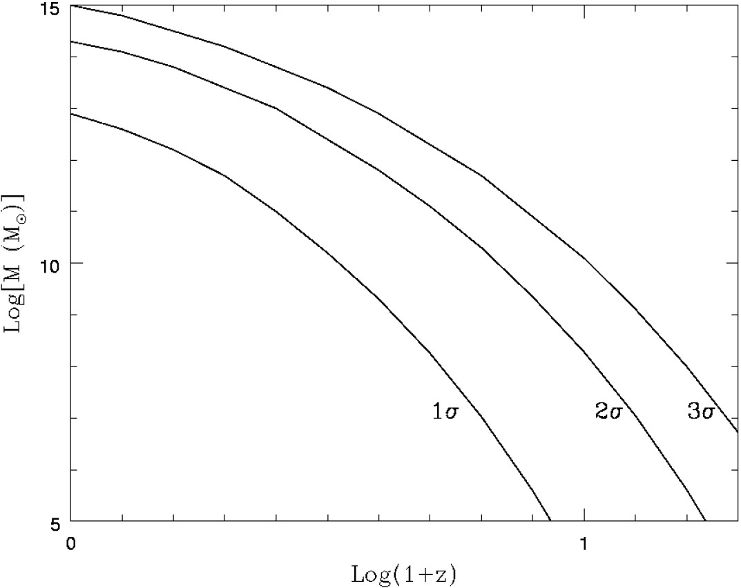Figure 7. Collapse redshifts of spherical top-hat 1, 2 and 3 perturbations in a CDM cosmology with 8 = 0.9. Note that galaxy-sized (M ~ 108 - 1013 M) 1 halos collapse in a redshift range, from z ~ 3.5 to z = 0, respectively; the corresponding ages are from ~ 1.9 to 13.8 Gyr, respectively.

The problem of cosmological gravitational clustering is very complex due to non-linearity, lack of symmetry and large dynamical range. Analytical and semi-analytical approaches provide illuminating results but numerical N-body simulations are necessary to tackle all the aspects of this problem. In the last 20 years, the "industry" of numerical simulations had an impressive development. The first cosmological simulations in the middle 80s used a few 10⁴ particles (e.g., [36]). The currently largest simulation (called the Millenium simulation [111]) uses ~ 10¹⁰ particles! A main effort is done to reach larger and larger dynamic ranges in order to simulate encompassing volumes large enough to contain representative populations of all kinds of halos (low mass and massive ones, in low- and high-density environments, high-peak rare halos), yet resolving the inner structure of individual halos.

Halo mass function

The CDM halo mass function (comoving number density of halos of different masses at a given epoch z, n(M, z)) obtained in the N-body simulations is consistent with the P-S function in general, which is amazing given the approximate character of the P-S analysis. However, in more detail, the results of large N-body simulations are better fitted by modified P-S analytical functions, as the one derived in [103] and showed in Fig. 8. Using the Millennium simulation, the halo mass function has been accurately measured in the range that is well sampled by this run (z 12, M 1.7 × 10¹⁰ M h^-1). The mass function is described by a power law at low masses and an exponential cut-off at larger masses. The "cut-off", most typical mass, increases with time and is related to the hierarchical evolution of the 1 halos shown in Fig. 7. The halo mass function is the starting point for modeling the luminosity function of galaxies. From Fig. 8 we see that the evolution of the abundances of massive halos is much more pronounced than the evolution of less massive halos. This is why observational studies of abundance of massive galaxies or cluster of galaxies at high redshifts provide a sharp test to theories of cosmic structure formation. The abundance of massive rare halos at high redshifts are for example a strong function of the fluctuation field primordial statistics (Gaussianity or non-Gaussianity).

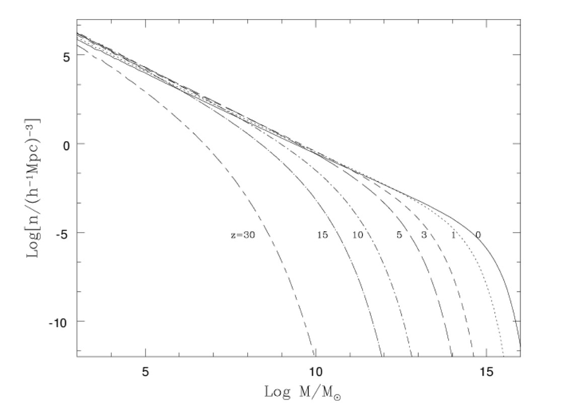Figure 8. Evolution of the comoving number density of collapsed halos (P-S mass function) according to the ellipsoidal modification by [103]. Note that the "cut-off" mass grows with time. Most of the mass fraction in collapsed halos at a given epoch are contained in halos with masses around the "cut-off" mass.

Subhalos. An important result of N-body simulations is the existence of subhalos, i.e. halos inside the virial radius of larger halos, which survived as self-bound entities the gravitational collapse of the higher level of the hierarchy. Of course, subhalos suffer strong mass loss due to tidal stripping, but this is probably not relevant for the luminous galaxies formed in the innermost regions of (sub)halos. This is why in the case of subhalos, the maximum circular velocity V_m (attained at radii much smaller than the virial radius) is used instead of the virial mass. The V_m distribution of subhalos inside cluster-sized and galaxy-sized halos is similar [83]. This distribution agrees with the distribution of galaxies seen in clusters, but for galaxy-sized halos the number of subhalos overwhelms by 1-2 orders of magnitude the observed number of satellite galaxies around galaxies like Milky Way and Andromeda [70, 83].

Fig. 9 (right side) shows the subhalo cumulative V_m-distribution for a CDM Milky Way-like halo compared to the observed satellite V_m-distribution. In this Fig. are also shown the V_m-distributions obtained for the same Milky-Way halo but using the power spectrum of three WDM models with particle masses m_X 0.6, 1, and 1.7 KeV. The smaller m_X, the larger is the free-streaming (filtering) scale, R_f, and the more substructure is washed out (see Section 3.2). In the left side of Fig. 9 is shown the DM distribution inside the Milky-Way halo simulated by using a CDM power spectrum (top) and a WDM power spectrum with m_X 1 KeV (sterile neutrino, bottom). For a student it should be exciting to see with her(his) own eyes this tight connection between micro- and macro-cosmos: the mass of the elemental particle determines the structure and substructure properties of galaxy halos!

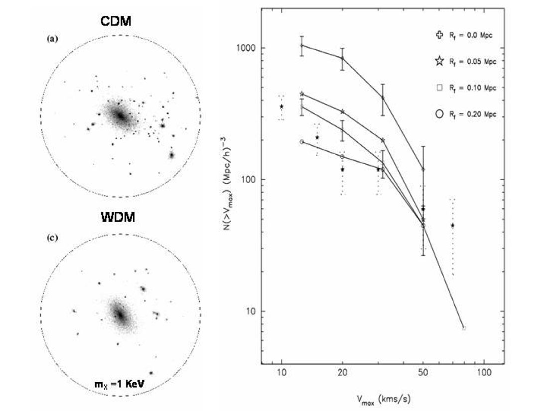Figure 9. Dark matter distribution in a sphere of 400 Mpch-1 of a simulated Galaxy-sized halo with CDM (a) and WDM (mX = 1 KeV, b). The substructure in the latter case is significantly erased. Right panel shows the cumulative maximum Vc distribution for both cases (open crosses and squares, respectively) as well as for an average of observations of satellite galaxies in our Galaxy and in Andromeda (dotted error bars). Adapted from [31].

High-resolution N-body simulations [87] and semi-analytical techniques (e.g., [3]) allowed to answer the following questions: How is the inner mass distribution in CDM halos? Does this distribution depend on mass? How universal is it? The two-parameter density profile established in [87] (the Navarro-Frenk-White, NFW profile) departs from a single power law, and it was proposed to be universal and not depending on mass. In fact the slope (r) -d log(r) / d logr of the NFW profile changes from -1 in the center to -3 in the periphery. The two parameters, a normalization factor, _s and a shape factor, r_s, were found to be related in a such a way that the profile depends only on one shape parameter that could be expressed as the concentration, c_NFW r_s / R_v. The more massive the halo, the less concentrated on the average. For the CDM model, c 20-5 for M ~ 2 × 10⁸ - 2 × 10¹⁵ M h^-1, respectively [42]. However, for a given M, the scatter of c_NFW is large ( 30 - 40%), and it is related to the halo formation history [3, 21, 125] (see below). A significant fraction of halos depart from the NFW profile. These are typically not relaxed or disturbed by companions or external tidal forces.

Is there a "cusp" crisis? More recently, it was found that the inner density profile of halos can be steeper than = -1 (e.g. [84]). However, it was shown that in the limit of resolution, never is as steep a -1.5 [88]. The inner structure of CDM halos can be tested in principle with observations of (i) the inner rotation curves of DM dominated galaxies (Irr dwarf and LSB galaxies; the inner velocity dispersion of dSph galaxies is also being used as a test ), and (ii) strong gravitational lensing and hot gas distribution in the inner regions of clusters of galaxies. Observations suggest that the DM distribution in dwarf and LSB galaxies has a roughly constant density core, in contrast to the cuspy cores of CDM halos (the literature on this subject is extensive; see for recent results [37, 50, 107, 128] and more references therein). If the observational studies confirm that halos have constant-density cores, then either astrophysical mechanisms able to expand the halo cores should work efficiently or the CDM scenario should be modified. In the latter case, one of the possibilities is to introduce weakly self-interacting DM particles. For small cross sections, the interaction is effective only in the more dense inner regions of galaxies, where heat inflow may expand the core. However, the gravo-thermal catastrophe can also be triggered. In [32] it was shown that in order to avoid the gravo-thermal instability and to produce shallow cores with densities approximately constant for all masses, as suggested by observations, the DM cross section per unit of particle mass should be _DM / m_X = 0.5 - 1.0 v₁₀₀^-1 cm² / gr, where v₁₀₀ is the relative velocity of the colliding particles in unities of 100 km/s; v₁₀₀ is close to the halo maximum circular velocity, V_m.

The DM mass distribution was inferred from the rotation curves of dwarf and LSB galaxies under the assumptions of circular motion, halo spherical symmetry, the lack of asymmetrical drift, etc. In recent studies it was discussed that these assumptions work typically in the sense of lowering the observed inner rotation velocity [59, 100, 118]. For example, in [118] it is demonstrated that non-circular motions (due to a bar) combined with gas pressure support and projection effects systematically underestimate by up to 50% the rotation velocity of cold gas in the central 1 kpc region of their simulated dwarf galaxies, creating the illusion of a constant density core.

Mass-velocity relation. In a very simplistic analysis, it is easy to find that M V_c³ if the average halo density _h does not depend on mass. On one hand, V_c (GM / R)^1/2, and on the other hand, _h M / R³, so that V_c M^1/3 _h^1/6. Therefore, for _h = const, M V_c³. We have seen in Section 3.2 that the CDM perturbations at galaxy scales have similar amplitudes (actually _M lnM) due to the stangexpansion effect in the radiation-dominated era. This implies that galaxy-sized perturbations collapse within a small range of epochs attaining more or less similar average densities. The CDM halos actually have a mass distribution that translates into a circular velocity profile V_c(r). The maximum of this profile, V_m, is typically the circular velocity that characterizes a given halo of virial mass M. Numerical and semi-numerical results show that (CDM model):

(14)

Assuming that the disk infrared luminosity L_IR M, and that the disk maximum rotation velocity V_rot,m V_m, one obtains that L_IR V_rot,m^3.2, amazingly similar to the observed infrared Tully-Fisher relation [116], one of the most robust and intriguingly correlations in the galaxy world! I conclude that this relation is a clear imprint of the CDM power spectrum of fluctuations.

Mass assembling histories

One of the key concepts of the hierarchical clustering scenario is that cosmic structures form by a process of continuous mass aggregation, opposite to the monolithic collapse scenario. The mass assembly of CDM halos is characterized by the mass aggregation history (MAH), which can alternate smooth mass accretion with violent major mergers. The MAH can be calculated by using semi-analytical approaches based on extensions of the P-S formalism. The main idea lies in the estimate of the conditional probability that given a collapsed region of mass M₀ at z₀, a region of mass M₁ embedded within the volume containing M₀, had collapsed at an earlier epoch z₁. This probability is calculated based on the excursion set formalism starting from a Gaussian density field characterized by an evolving mass variance _M [17, 73]. By using the conditional probability and random trials at each temporal step, the "backward" MAHs corresponding to a fixed mass M₀ (defined for instance at z = 0) can be traced. The MAHs of isolated halos by definition decrease toward the past, following different tracks (Fig. 10), sometimes with abrupt big jumps that can be identified as major mergers in the halo assembly history.

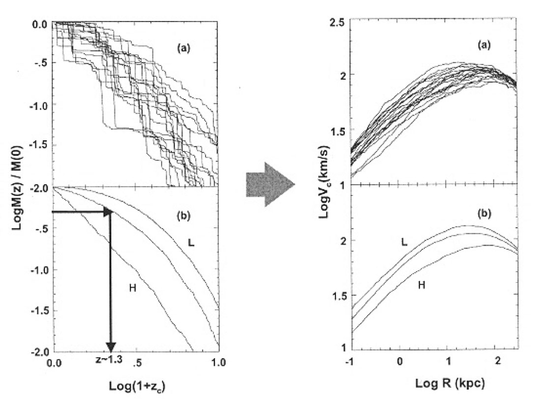Figure 10. Upper panels (a). A score of random halo MAHs for a present-day virial mass of 3.5 × 1011 M and the corresponding circular velocity profiles of the virialized halos. Lower panels (b). The average MAH and two extreme deviations from 104 random MAHs for the same mass as in (a), and the corresponding halo circular velocity profiles. The MAHs are diverse for a given mass and the Vc (mass) distribution of the halos depend on the MAH. Adapted from [45].

To characterize typical behaviors of the halo MAHs, one may calculate the average MAH for a given virial mass M₀, for a given "population" of halos selected by its environment, etc. In the left panels of Fig. 10 are shown 20 individual MAHs randomly selected from 10⁴ trials for M₀ = 3.5 × 10¹¹ M in a CDM cosmology [45]. In the bottom panel are plotted the average MAH from these 10⁴ trials as well as two extreme deviations from the average. The average MAHs depend on mass: more massive halos have a more extended average MAH, i.e. they aggregate a given fraction of M₀ latter than less massive halos. It is a convention to define the typical halo formation redshift, z_f, when half of the current halo mass M₀ has been aggregated. For instance, for the CDM cosmology the average MAHs show that z_f 2.2, 1.2 and 0.7 for M₀ = 10¹⁰ M, 10¹² M and 10¹⁴ M, respectively. A more physical definition of halo formation time is when the halo maximum circular velocity V_m attains its maximum value. After this epoch, the mass can continue growing, but the inner gravitational potential of the system is already set.

Right panels of Fig. 10 show the present-day halo circular velocity profiles, V_c(r), corresponding to the MAHs plotted in the left panels. The average V_c(r) is well described by the NFW profile. There is a direct relation between the MAH and the halo structure as described by V_c(r) or the concentration parameter. The later the MAH, the more extended is V_c(r) and the less concentrated is the halo [3, 125]. Using high-resolution simulations some authors have shown that the halo MAH presents two regimes: an early phase of fast mass aggregation (mainly by major mergers) and a late phase of slow aggregation (mainly by smooth mass accretion) [133, 75]. The potential well of a present-day halo is set mainly at the end of the fast, major-merging driven, growth phase.

From the MAHs we may infer: (i) the mass aggregation rate evolution of halos (halo mass aggregated per unit of time at different z's), and (ii) the major merging rates of halos (number of major mergers per unit of time per halo at different z's). These quantities should be closely related to the star formation rates of the galaxies formed within the halos as well as to the merging of luminous galaxies and pair galaxy statistics. By using the CDM model, several studies showed that most of the mass of the present-day halos has been aggregated by accretion rather than major mergers (e.g., [85]). Major merging was more frequent in the past [55], and it is important for understanding the formation of massive galaxy spheroids and the phenomena related to this process like QSOs, supermassive black hole growth, obscured star formation bursts, etc. Both the mass aggregation rate and major merging rate histories depend strongly on environment: the denser the environment, the higher is the merging rate in the past. However, in the dense environments (group and clusters) form typically structures more massive than in the less dense regions (field and voids). Once a large structure virializes, the smaller, galaxy-sized halos become subhalos with high velocity dispersions: the mass growth of the subhalos is truncated, or even reversed due to tidal stripping, and the merging probability strongly decreases. Halo assembling (and therefore, galaxy assembling) definitively depends on environment. Overall, by integrating the MAHs of the whole galaxy-sized CDM halo population in a given volume, the general result is that the peak in halo assembling activity was at z 1-2. After these redshifts, the global mass aggregation rate strongly decreases (e.g., [121].

To illustrate the driving role of DM processes in galaxy evolution, I mention briefly here two concrete examples:

1). Distributions of present-day specific mass aggregation rate, ( / M)₀, and halo lookback formation time, T_1/2. For a CDM model, these distributions are bimodal, in particular the former. We have found that roughly 40% of halos (masses larger than 10¹¹ M h^-1) have ( / M)₀ 0; they are basically subhalos. The remaining 60% present a broad distribution of ( / M)₀ > 0 peaked at 0.04 Gyr^-1. Moreover, this bimodality strongly changes with large-scale environment: the denser is the environment the, higher is the fraction of halos with ( / M)₀ 0. It is interesting enough that similar fractions and dependences on environment are found for the specific star formation rates of galaxies in large statistical surveys (Section 2.3); the situation is similar when confronting the distributions of T_1/2 and observed colors. Therefore, it seems that the the main driver of the observed bimodalities in z = 0 specific star formation rate and color of galaxies is the nature of the CDM halo mass aggregation process. Astrophysical processes of course are important but the main body of the bimodalities can be explained just at the level of DM processes.

2. Major merging rates. The observational inference of galaxy major merging rates is not an easy task. The two commonly used methods are based on the statistics of galaxy pairs (pre-mergers) and in the morphological distortions of ellipticals (post-mergers). The results show that the merging rate increases as (1 + z)^x, with x ~ 0-4. The predicted major merging rates in the CDM scenario agree roughly with those inferred from statistics of galaxy pairs. From the fraction of normal galaxies in close companions (with separations less than 50 kpch^-1) inferred from observations at z = 0 and z = 0.3 [91], and assuming an average merging time of ~ 1 Gyr for these separations, we estimate that the major merging rate at the present epoch is ~ 0.01 Gyr^-1 for halos in the range of 0.1 - 2.0 × 10¹² M, while at z = 0.3 the rate increased to ~ 0.018 Gyr^-1. These values are only slightly lower than predictions for the CDM model.

Angular momentum

The origin of the angular momentum (AM) is a key ingredient in theories of galaxy formation. Two mechanisms of AM acquirement were proposed for the CDM halos (e.g., [93, 22, 78]): 1. tidal torques of the surrounding shear field when the perturbation is still in the linear regime, and 2. transfer of orbital AM to internal AM in major and minor mergers of collapsed halos. The angular momentum of DM halos is parametrized in terms of the dimensionless spin parameter J (E)^1/2 / (GM^5/2, where J is the modulus of the total angular momentum and E is the total (kinetic plus potential). It is easy to show that can be interpreted as the level of rotational support of a gravitational system, = / _sup, where is the angular velocity of the system and _sup is the angular velocity needed for the system to be rotationally supported against gravity (see [90]).

For disk and elliptical galaxies, ~ 0.4-0.8 and ~ 0.01-0.05, respectively. Cosmological N-body simulations showed that the CDM halo spin parameter is log-normal distributed, with a median value 0.04 and a standard deviation 0.5; this distribution is almost independent from cosmology. A related quantity, but more straightforward to compute is ' J / [(2)^1/2 M V_v R_v] [22], where R_v is the virial radius and V_v the circular velocity at this radius. Recent simulations show that (', _') (0.035,0.6), though some variations with environment and mass are measured [5]. The evolution of the spin parameter depends on the AM acquirement mechanism. In general, a significant systematical change of with time is not expected, but relatively strong changes are measured in short time steps, mainly after merging of halos, when increases.

How is the internal AM distribution in CDM halos? Bullock et al. [22] found that in most of cases this distribution can be described by a simple (universal) two-parameter function that departs significantly from the solid-body rotation distribution. In addition, the spatial distribution of AM in CDM halos tends to be cylindrical, being well aligned for 80% of the halos, and misaligned at different levels for the rest. The mass distribution of the galaxies formed within CDM halos, under the assumption of specific AM conservation, is established by , the halo AM distribution, and its alignment.

4.2. Non-baryonic dark matter candidates

The non-baryonic DM required in cosmology to explain observations and cosmic structure formation should be in form of elemental or scalar field particles or early formed quark nuggets. Modifications to fundamental physical theories (modified Newtonian Dynamics, extra-dimensions, etc.) are also plausible if DM is not discovered.

There are several docens of predicted elemental particles as DM candidates. The list is reduced if we focus only on well-motivated exotic particles from the point of view of particle physics theory alone (see for a recent review [53]). The most popular particles beyond the standard model are the supersymmetric (SUSY) particles in supersymmetric extensions of the Standard Model of particle physics. Supersymmetry is a new symmetry of space-time introduced in the process of unifying the fundamental forces of nature (including gravity). An excellent CDM candidate is the lightest stable SUSY particle under the requirement that superpartners are only produced or destroyed in pairs (called R-parity conservation). This particle called neutralino is weakly interacting and massive (WIMP). Other SUSY particles are the gravitino and the sneutrino; they are of WDM type. The predicted masses for neutralino range from ~ 30 to 5000 GeV. The cosmological density of neutralino (and of other thermal WIMPs) is naturally as required when their interaction cross section is of the order of a weak cross section. The latter gives the possibility to detect neutralinos in laboratory.

The possible discovery of WIMPs relies on two main techniques:

(i) Direct detections. The WIMP interactions with nuclei (elastic scattering) in ultra-low-background terrestrial targets may deposit a tiny amount of energy (< 50 keV) in the target material; this kinetic energy of the recoiling nucleus is converted partly into scintillation light or ionization energy and partly into thermal energy. Dozens of experiments worldwide -of cryogenic or scintillator type, placed in mines or underground laboratories, attempt to measure these energies. Predicted event rates for neutralinos range from 10^-6 to 10 events per kilogram detector material and day. The nuclear recoil spectrum is featureless, but depends on the WIMP and target nucleus mass. To convincingly detect a WIMP signal, a specific signature from the galactic halo particles is important. The Earth's motion through the galaxy induces both a seasonal variation of the total event rate and a forward-backward asymmetry in a directional signal. The detection of structures in the dark velocity space, as those predicted to be produced by the Sagittarius stream, is also an specific signature from the Galactic halo; directional detectors are needed to measure this kind of signatures.

The DAMA collaboration reported a possible detection of WIMP particles obeying the seasonal variation; the most probable value of the WIMP mass was ~ 60 GeV. However, the interpretation of the detected signal as WIMP particles is controversial. The sensitivity of current experiments (e.g., CDMS and EDEL-WEISS) limit already the WIMP-proton spin-independent cross sections to values 2 × 10^-42 - 10^-40 cm^-2 for the range of masses ~ 50 - 10⁴ GeV, respectively; for smaller masses, the cross-section sensitivities are larger, and WIMP signals were not detected. Future experiments will be able to test the regions in the cross-section-WIMP mass diagram, where most of models make certain predictions.

(ii) Indirect detections. We can search for WIMPS by looking for the products of their annihilation. The flux of annihilation products is proportional to the square of the WIMP density, thus regions of interest are those where the WIMP concentration is relatively high. There are three types of searches according to the place where WIMP annihilation occur: (i) in the Sun or the Earth, which gives rise to a signal in high-energy neutrinos; (ii) in the galactic halo, or in the halo of external galaxies, which generates -rays and other cosmic rays such as positrons and antiprotons; (iii) around black holes, specially around the black hole at the Galactic Center. The predicted radiation fluxes depend on the particle physics model used to predict the WIMP candidate and on astrophysical quantities such as the dark matter halo structure, the presence of sub-structure, and the galactic cosmic ray diffusion model.

Most of WIMPS were in thermal equilibrium in the early Universe (thermal relics). Particles which were produced by a non-thermal mechanism and that never had the chance of reaching thermal equilibrium are called non-thermal relics (e.g., axions, solitons produced in phase transitions, WIMPZILLAs produced gravitationally at the end of inflation). From the side of WDM, the most popular candidate are the ~ 1 KeV sterile neutrinos. A sterile neutrino is a fermion that has no standard model interactions other than a coupling to the standard neutrinos through their mass generation mechanism. Cosmological probes, mainly the power spectrum of Ly forest at high redshifts, constrain the mass of the sterile neutrino to values larger than ~ 2 KeV.

¹¹ The spherical top-hat model refers to the exact calculation of the collapse of a uniform spherical density perturbation in an otherwise uniform Universe; the dynamics of such a region is the same of a closed Universe. The solution of the equations of motion shows that the perturbation at the beginning expands as the background Universe (proportional to a), then it reaches a maximum expansion (size) in a time t_max, and since that moment the perturbation separates of the expanding background, collapsing in a time t_col = 2t_max. Back.

¹² The mathematical solution gives that the spherical perturbed region collapses into a point (a black hole) after reaching its maximum expansion. However, real perturbations are lumpy and the particle orbits are not perfectly radial. In this situation, during the collapse the structure comes to a dynamical equilibrium under the influence of large scale gravitational potential gradients, a process named by the oxymoron "violent relaxation" (see e.g. [14]); this is a typical collective phenomenon. The end result is a system that satisfies the virial theorem: for a self-gravitating system this means that the internal kinetic energy is half the (negative) gravitational potential energy. Gravity is supported by the velocity dispersion of particles or lumps. The collapse factor is roughly 1/2, i.e. the typical virial radius R_v of the collapsed structure is 0.5 the radius of the perturbation at its maximum expansion. Back.