3. COSMIC STRUCTURE FORMATION

In the previous section we have learn that galaxy formation and evolution are definitively related to cosmological conditions. Cosmology provides the theoretical framework for the initial and boundary conditions of the cosmic structure formation models. At the same time, the confrontation of model predictions with astronomical observations became the most powerful testbed for cosmology. As a result of this fruitful convergence between cosmology and astronomy, there emerged the current paradigmatic scenario of cosmic structure formation and evolution of the Universe called Cold Dark Matter (CDM). The CDM scenario integrates nicely: (1) cosmological theories (Big Bang and Inflation), (2) physical models (standard and extensions of the particle physics models), (3) astrophysical models (gravitational cosmic structure growth, hierarchical clustering, gastrophysics), and (4) phenomenology (CMBR anisotropies, non-baryonic DM, repulsive dark energy, flat geometry, galaxy properties).

Nowadays, cosmology passed from being the Cinderella of astronomy to be one of the highest precision sciences. Let us consider only the Inflation/Big Bang cosmological models with the F-R-W metric and adiabatic perturbations. The number of parameters that characterize these models is high, around 15 to be more precise. No single cosmological probe constrain all of these parameters. By using multiple data sets and probes it is possible to constrain with precision several of these parameters, many of which correlate among them (degeneracy). The main cosmological probes used for precision cosmology are the CMBR anisotropies, the type-Ia SNe and long Gamma-Ray Bursts, the Ly power spectrum, the large-scale power spectrum from galaxy surveys, the cluster of galaxies dynamics and abundances, the peculiar velocity surveys, the weak and strong lensing, the baryonic acoustic oscillation in the large-scale galaxy distribution. There is a model that is systematically consistent with most of these probes and one of the goals in the last years has been to improve the error bars of the parameters for this 'concordance' model. The geometry in the concordance model is flat with an energy composition dominated in ~ 2/3 by the cosmological constant (generically called Dark Energy), responsible for the current accelerated expansion of the Universe. The other ~ 1/3 is matter, but ~ 85% of this 1/3 is in form of non-baryonic DM. Table 2 presents the central values of different parameters of the CDM cosmology from combined model fittings to the recent 3-year WMAP CMBR and several other cosmological probes [109] (see the WMAP website).

Table 2. Constraints to the parameters of the CDM model

Parameter	Constraint
Total density	= 1
Dark Energy density	= 0.74
Dark Matter density	DM = 0.216
Baryon Matter dens.	B = 0.044
Hubble constant	h = 0.71
Age	13.8 Gyr
Power spectrum norm.	8 = 0.75
Power spectrum index	ns(0.002) = 0.94

3.1. Origin of fluctuations

The Big Bang ⁴ is now a mature theory, based on well established observational pieces of evidence. However, the Big Bang theory has limitations. One of them is namely the origin of fluctuations that should give rise to the highly inhomogeneous structure observed today in the Universe, at scales of less than ~ 200 Mpc. The smaller the scales, the more clustered is the matter. For example, the densities inside the central regions of galaxies, within the galaxies, cluster of galaxies, and superclusters are about 10¹¹, 10⁶, 10³ and few times the average density of the Universe, respectively.

The General Relativity equations that describe the Universe dynamics in the Big Bang theory are for an homogeneous and isotropic fluid (Cosmological Principle); inhomogeneities are not taken into account in this theory "by definition". Instead, the concept of fluctuations is inherent to the Inflationary theory introduced in the early 80's by A. Guth and A. Linde namely to overcome the Big Bang limitations. According to this theory, at the energies of Grand Unification ( 10¹⁴ GeV or T 10²⁷ K!), the matter was in the state known in quantum field theory as vacuum. Vacuum is characterized by quantum fluctuations -temporary changes in the amount of energy in a point in space, arising from Heisenberg uncertainty principle. For a small time interval t, a virtual particle-antiparticle pair of energy E is created (in the GU theory, the field particles are supposed to be the X- and Y-bossons), but then the pair disappears so that there is no violation of energy conservation. Time and energy are related by E t h / 2. The vacuum quantum fluctuations are proposed to be the seeds of present-day structures in the Universe.

How is that quantum fluctuations become density inhomogeneities? During the inflationary period, the expansion is described approximately by the de Sitter cosmology, a e^Ht, H / a is the Hubble parameter and it is constant in this cosmology. Therefore, the proper length of any fluctuation grows as _p e^Ht. On the other hand, the proper radius of the horizon for de Sitter metric is equal to c / H = const, so that initially causally connected (quantum) fluctuations become suddenly supra-horizon (classical) perturbations to the spacetime metric. After inflation, the Hubble radius grows proportional to ct, and at some time a given curvature perturbation cross again the horizon (becomes causally connected, _p < L_H). It becomes now a true density perturbation. The interesting aspect of the perturbation 'trip' outside the horizon is that its amplitude remains roughly constant, so that if the amplitude of the fluctuations at the time of exiting the horizon during inflation is constant (scale invariant), then their amplitude at the time of entering the horizon should be also scale invariant. In fact, the computation of classical perturbations generated by a quantum field during inflation demonstrates that the amplitude of the scalar fluctuations at the time of crossing the horizon is nearly constant, _H const. This can be understood on dimensional grounds: due to the Heisenberg principle / t const, where t H^-1. Therefore, _H H, but H is roughly constant during inflation, so that _H const.

3.2. Gravitational evolution of fluctuations

The CDM scenario assumes the gravitational instability paradigm: the cosmic structures in the Universe were formed as a consequence of the growth of primordial tiny fluctuations (for example seeded in the inflationary epochs) by gravitational instability in an expanding frame. The fluctuation or perturbation is characterized by its density contrast,

(1)

where is the average density of the Universe and is the perturbation density. At early epochs, << 1 for perturbation of all scales, otherwise the homogeneity condition in the Big Bang theory is not anymore obeyed. When << 1, the perturbation is in the linear regime and its physical size grows with the expansion proportional to a(t). The perturbation analysis in the linear approximation shows whether a given perturbation is stable ( ~ const or even 0) or unstable ( grows). In the latter case, when 1, the linear approximation is not anymore valid, and the perturbation "separates" from the expansion, collapses, and becomes a self-gravitating structure. The gravitational evolution in the non-linear regime is complex for realistic cases and is studied with numerical N-body simulations. Next, a pedagogical review of the linear evolution of perturbations is presented. More detailed explanations on this subject can be found in the books [72, 94, 90, 30, 77, 92].

Relevant times and scales.

The important times in the problem of linear gravitational evolution of perturbations are: (a) the epoch when inflation finished (t_inf 10^-34 s, at this time the primordial fluctuation field is established); (b) the epoch of matter-radiation equality t_eq (corresponding to a_eq 1/3.9 × 10⁴(₀ h²), before t_eq the dynamics of the universe is dominated by radiation density, after t_eq dominates matter density); (c) the epoch of recombination t_rec, when radiation decouples from baryonic matter (corresponding to a_rec=1/1080, or t_rec 3.8 × 10⁵yr for the concordance cosmology).

Scales: first of all, we need to characterize the size of the perturbation. In the linear regime, its physical size expands with the Universe: _p = a(t) ₀, where ₀ is the comoving size, by convention fixed (extrapolated) to the present epoch, a(t₀) = 1. In a given (early) epoch, the size of the perturbation can be larger than the so-called Hubble radius, the typical radius over which physical processes operate coherently (there is causal connection): L_H (a / )^-1 = H^-1 = n^-1 ct. For the radiation or matter dominated cases, a(t) tⁿ, with n = 1/2 and n = 2/3, respectively, that is n < 1. Therefore, L_H grows faster than _p and at a given "crossing" time t_cross, _p < L_H. Thus, the perturbation is supra-horizon sized at epochs t < t_cross and sub-horizon sized at t > t_cross. Notice that if n > 1, then at some time the perturbation "exits" the Hubble radius. This is what happens in the inflationary epoch, when a(t) e^t: causally-connected fluctuations of any size are are suddenly "taken out" outside the Hubble radius becoming causally disconnected.

For convenience, in some cases it is better to use masses instead of sizes. Since in the linear regime << 1 ( ), then M _M(a) ³, where is the size of a given region of the Universe with average matter density _M. The mass of the perturbation, M_p, is invariant.

Supra-horizon sized perturbations.

In this case, causal, microphysical processes are not possible, so that it does not matter what perturbations are made of (baryons, radiation, dark matter, etc.); they are in general just perturbations to the metric. To study the gravitational growth of metric perturbations, a General Relativistic analysis is necessary. A major issue in carrying out this program is that the metric perturbation is not a gauge invariant quantity. See e.g., [72] for an outline of how E. Lifshitz resolved brilliantly this difficult problem in 1946. The result is quite simple and it shows that the amplitude of metric perturbations outside the horizon grows kinematically at different rates, depending on the dominant component in the expansion dynamics. For the critical cosmological model (at early epochs all models approach this case), the growing modes of metric perturbations according to what dominates the background are:

(2) (3)

Sub-horizon sized perturbations.

Once perturbations are causally connected, microphysical processes are switched on (pressure, viscosity, radiative transport, etc.) and the gravitational evolution of the perturbation depends on what it is made of. Now, we deal with true density perturbations. For them applies the classical perturbation analysis for a fluid, originally introduced by J. Jeans in 1902, in the context of the problem of star formation in the ISM. But unlike in the ISM, in the cosmological context the fluid is expanding. What can prevent the perturbation amplitude from growing gravitationally? The answer is pressure support. If the fluid pressure gradient can re-adjust itself in a timescale t_press smaller than the gravitational collapse timescale, t_grav, then pressure prevents the gravitational growth of . Thus, the condition for gravitational instability is:

(4)

where is the density of the component that is most gravitationally dominant in the Universe, and v is the sound speed (collisional fluid) or velocity dispersion (collisionless fluid) of the perturbed component. In other words, if the perturbation scale is larger than a critical scale _J ~ v(G )^-1/2, then pressure loses, gravity wins.

The perturbation analysis applied to the hydrodynamical equations of a fluid at rest shows that grows exponentially with time for perturbations obeying the Jeans instability criterion _p > _J, where the exact value of _J is v( / G )^1/2. If _p < _J, then the perturbations are described by stable gravito-acustic oscillations. The situation is conceptually similar for perturbations in an expanding cosmological fluid, but the growth of in the unstable regime is algebraical instead of exponential. Thus, the cosmic structure formation process is relatively slow. Indeed, the typical epochs of galaxy and cluster of galaxies formation are at redshifts z ~ 1 - 5 (ages of ~ 1.2 - 6 Gyrs) and z < 1 (ages larger than 6 Gyrs), respectively.

Baryonic matter. The Jeans instability analysis for a relativistic (plasma) fluid of baryons ideally coupled to radiation and expanding at the rate H = / a shows that there is an instability critical scale _J = v(3 / 8G )^1/2, where the sound speed for adiabatic perturbations is v = p / = c / (3)^1/2; the latter equality is due to pressure radiation. At the epoch when radiation dominates, = _r a^-4 and then _J a² ct. It is not surprising that at this epoch _J approximates the Hubble scale L_H ct (it is in fact ~ 3 times larger). Thus, perturbations that might collapse gravitationally are in fact outside the horizon, and those that already entered the horizon, have scales smaller than _J: they are stable gravito-acoustic oscillations. When matter dominates, = _M a^-3, and a t^2/3. Therefore, _J a t^2/3 L_H, but still radiation is coupled to baryons, so that radiation pressure is dominant and _J remains large. However, when radiation decouples from baryons at t_rec, the pressure support drops dramatically by a factor of P_r / P_b n_r T / n_b T 10⁸! Now, the Jeans analysis for a gas mix of H and He at temperature T_rec 4000 K shows that baryonic clouds with masses 10⁶ M can collapse gravitationally, i.e. all masses of cosmological interest. But this is literally too "ideal" to be true.

The problem is that as the Universe expands, radiation cools (T_r = T₀ a^-1) and the photon-baryon fluid becomes less and less perfect: the mean free path for scattering of photons by electrons (which at the same time are coupled electrostatically to the protons) increases. Therefore, photons can diffuse out of the bigger and bigger density perturbations as the photon mean free path increases. If perturbations are in the gravito-acoustic oscillatory regime, then the oscillations are damped out and the perturbations disappear. The "ironing out" of perturbations continues until the epoch of recombination. In a pioneering work, J. Silk [104] carried out a perturbation analysis of a relativistic cosmological fluid taking into account radiative transfer in the diffusion approximation. He showed that all photon-baryon perturbations of masses smaller than M_s are "ironed out" until t_rec by the (Silk) damping process. The first crisis in galaxy formation theory emerged: calculations showed that M_s is of the order of 10¹³ - 10¹⁴ M h^-1! If somebody (god, inflation, ...) seeded primordial fluctuations in the Universe, by Silk damping all galaxy-sized perturbation are "ironed out". ⁵

Non-baryonic matter. The gravito-acoustic oscillations and their damping by photon diffusion refer to baryons. What happens for a fluid of non-baryonic DM? After all, astronomers, since Zwicky in the 1930s, find routinely pieces of evidence for the presence of large amounts of DM in the Universe. As DM is assumed to be collisionless and not interacting electromagnetically, then the radiative or thermal pressure supports are not important for linear DM perturbations. However, DM perturbations can be damped out by free streaming if the particles are relativistic: the geodesic motion of the particles at the speed of light will iron out any perturbation smaller than a scale close to the particle horizon radius, because the particles can freely propagate from an overdense region to an underdense region. Once the particles cool and become non relativistic, free streaming is not anymore important. A particle of mass m_X and temperature T_X becomes non relativistic when k_B T_X ~ m_X c². Since T_X a^-1, and a t^1/2 when radiation dominates, one then finds that the epoch when a thermal-relic particle becomes non relativistic is t_nr m_X^-2. The more massive the DM particle, the earlier it becomes non relativistic, and the smaller are therefore the perturbations damped out by free streaming (those smaller than ~ ct; see Fig. 4). According to the epoch when a given thermal DM particle species becomes non relativistic, DM is called Cold Dark Matter (CDM, very early), Warm Dark Matter (WDM, early) and Hot Dark Matter (HDM, late) ⁶.

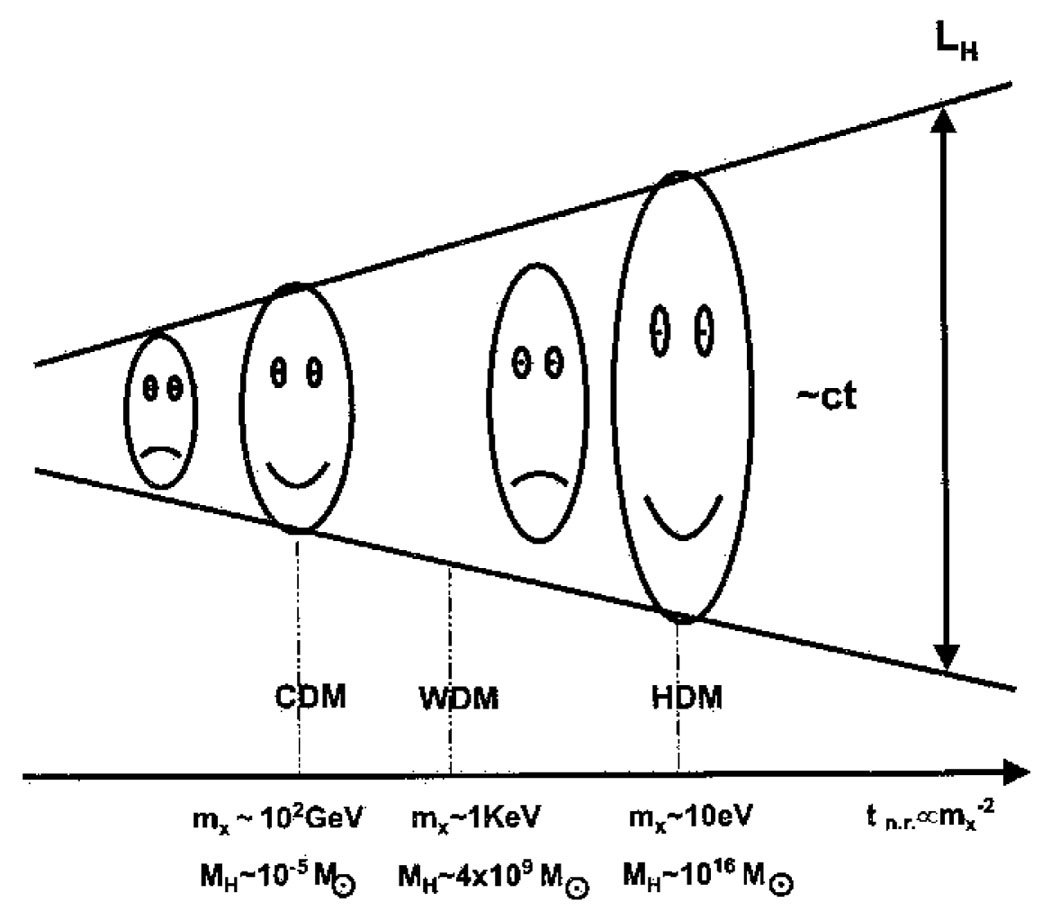Figure 4. Free-streaming damping kills perturbations of sizes roughly smaller than the horizon length if they are made of relativistic particles. The epoch tn.r. when thermal-coupled particles become non-relativistic is inverse proportional to the square of the particle mass mX. Typical particle masses of CDM, WDM and HDM are given together with the corresponding horizon (filtering) masses.

The only non-baryonic particles confirmed experimentally are (light) neutrinos (HDM). For neutrinos of masses ~ 1 - 10eV, free streaming attains to iron out perturbations of scales as large as massive clusters and superclusters of galaxies (see Fig. 4). Thus, HDM suffers the same problem of baryonic matter concerning galaxy formation ⁷. At the other extreme is CDM, in which case survive free streaming practically all scales of cosmological interest. This makes CDM appealing to galaxy formation theory. In the minimal CDM model, it is assumed that perturbations of all scales survive, and that CDM particles are collisionless (they do not self-interact). Thus, if CDM dominates, then the first step in galaxy formation study is reduced to the calculation of the linear and non-linear gravitational evolution of collisionless CDM perturbations. Galaxies are expected to form in the centers of collapsed CDM structures, called halos, from the baryonic gas, first trapped in the gravitational potential of these halos, and second, cooled by radiative (and turbulence) processes (see Section 5).

The CDM perturbations are free of any physical damping processes and in principle their amplitudes may grow by gravitational instability. However, when radiation dominates, the perturbation growth is stagnated by expansion. The gravitational instability timescale for sub-horizon linear CDM perturbations is t_grav ~ (G _DM)^-2, while the expansion (Hubble) timescale is given by t_exp ~ (G )^-2. When radiation dominates, _r and _r >> _M. Therefore t_exp << t_grav, that is, expansion is faster than the gravitational shrinking.

Fig. 5 resumes the evolution of primordial perturbations. Instead of spatial scales, in Fig. 5 are shown masses, which are invariant for the perturbations. We highlight the following conclusions from this plot: (1) Photon-baryon perturbations of masses < M_s are washed out (_B 0) as long as baryon matter is coupled to radiation. (2) The amplitude of CDM perturbations that enter the horizon before t_eq is "freezed-out" (_DM const) as long as radiation dominates; these are perturbations of masses smaller than M_H,eq 10¹³(_M h²)^-2 M, namely galaxy scales. (3) The baryons are trapped gravitationally by CDM perturbations, and within a factor of two in z, baryon perturbations attain amplitudes half that of _DM. For WDM or HDM perturbations, the free-streaming damping introduces a mass scale M_fs M_H,n.r. in Fig. 5, below which 0; M_fs increases as the DM mass particle decreases (Fig. 4).

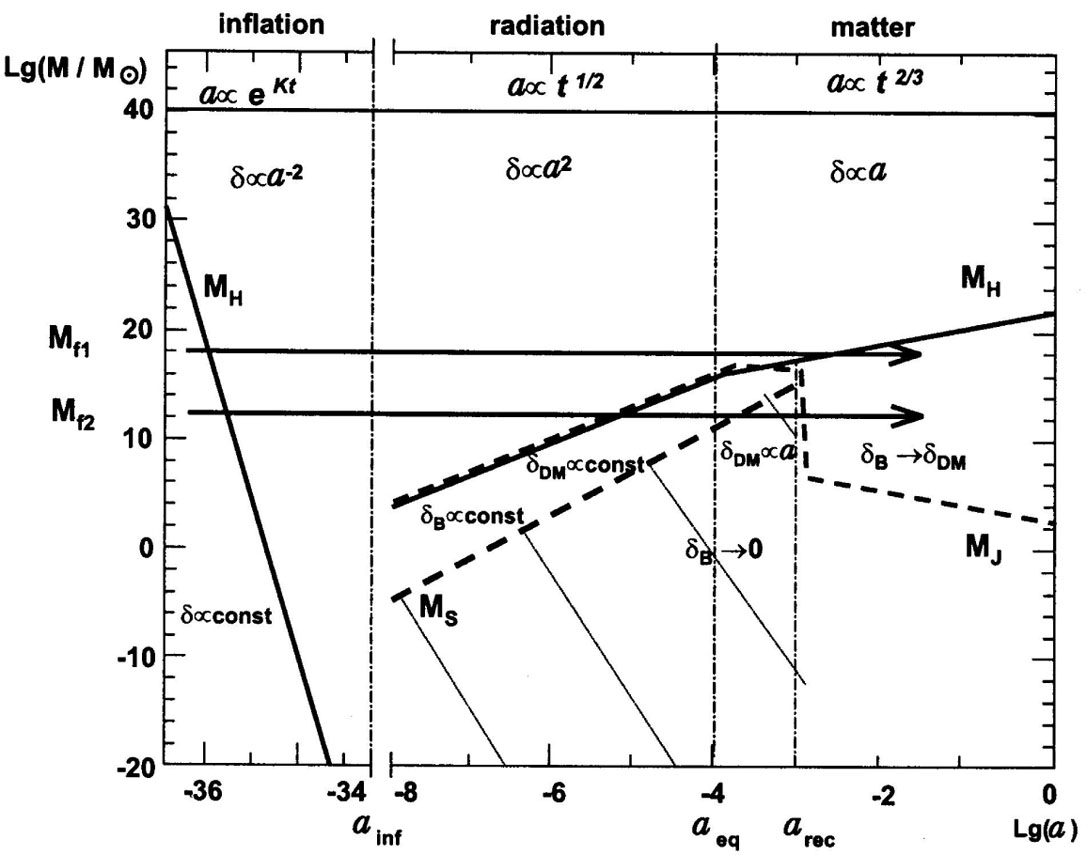Figure 5. Different evolutive regimes of perturbations . The suffixes "B" and "DM" are for baryon-photon and DM perturbations, respectively. The evolution of the horizon, Jeans and Silk masses (MH, MJ, and Ms) are showed. Mf1 and Mf2 are the masses of two perturbations. See text for explanations.

The processed power spectrum of perturbations. The exact solution to the problem of linear evolution of cosmological perturbations is much more complex than the conceptual aspects described above. Starting from a primordial fluctuation field, the perturbation analysis should be applied to a cosmological mix of baryons, radiation, neutrinos, and other non-baryonic dark matter components (e.g., CDM), at sub- and supra-horizon scales (the fluid assumption is relaxed). Then, coupled relativistic hydrodynamic and Boltzmann equations in a general relativity context have to be solved taking into account radiative and dissipative processes. The outcome of these complex calculations is the full description of the processed fluctuation field at the recombination epoch (when fluctuations at almost all scales are still in the linear regime). The goal is double and of crucial relevance in cosmology and astrophysics: 1) to predict the physical and statistical properties of CMBR anisotropies, which can be then compared with observations, and 2) to provide the initial conditions for calculating the non-linear regime of cosmic structure formation and evolution. Fortunately, there are now several public friendly-to-use codes that numerically solve the cosmological linear perturbation equations (e.g., CMBFast and CAMB ⁸).

The description of the density fluctuation field is statistical. As any random field, it is convenient to study perturbations in the Fourier space. The Fourier expansion of (x) is:

(5) (6)

The Fourier modes _k evolve independently while the perturbations are in the linear regime, so that the perturbation analysis can be applied to this quantity. For a Gaussian random field, any statistical quantity of interest can be specified in terms of the power spectrum P(k) |_k|², which measures the amplitude of the fluctuations at a given scale k ⁹. Thus, from the linear perturbation analysis we may follow the evolution of P(k). A more intuitive quantity than P(k) is the mass variance _M² <(M / M)_r²> of the fluctuation field. The physical meaning of _M is that of an rms density contrast on a given sphere of radius R associated to the mass M = V_W(R), where W(R) is a window (smoothing) function. The mass variance is related to P(k). By assuming a power law power spectrum, P(k) kⁿ, it is easy to show that

(7)

for 4 < n < -3 using a Gaussian window function. The question is: How the scaling law of perturbations, _M, evolves starting from an initial (_M)_i?

In the early 1970s, Harrison and Zel'dovich independently asked themselves about the functionality of _M (or the density contrast) at the time adiabatic perturbations cross the horizon, that is, if (_M)_H M^_H, then what is the value of _H? These authors concluded that -0.1 _H 0.2, i.e. _H 0 (n_H -3). If _H >> 0 (n_H >> -3), then _M for M 0; this means that for a given small mass scale M, the mass density of the perturbation at the time of becoming causally connected can correspond to the one of a (primordial) black hole. Hawking evaporation of black holes put a constraint on M_BH,prim 10¹⁵ g, which corresponds to _H 0.2, otherwise the -ray background radiation would be more intense than that observed. If _H << 0 (n_H << -3), then larger scales would be denser than the small ones, contrary to what is observed. The scale-invariant Harrison-Zel'dovich power spectrum, P_H(k) k^-3, is for perturbations at the time of entering the horizon. How should the primordial power spectrum P_i(k) = Ak_iⁿ or (_M)_i = BM^-_i (defined at some fixed initial time) be to produce such scale invariance? Since t_i until the horizon crossing time t_cross(M) for a given perturbation of mass M, _M(t) evolves as a(t)² (supra-horizon regime in the radiation era). At t_cross, the horizon mass M_H is equal by definition to M. We have seen that M_H a³ (radiation dominion), so that a_cross M_H^1/3 = M^1/3. Therefore,

(8)

i.e. _H = 2/3 - _i or n_H = n_i - 4. A similar result is obtained if the perturbation enters the horizon during the matter dominion era. From this analysis one concludes that for the perturbations to be scale invariant at horizon crossing (_H = 0 or n_H = -3), the primordial (initial) power spectrum should be P_i(k) = Ak¹ or (_M)_i M^-2/3 ₀^-2 (i.e. n_i = 1 and = 2/3; A is a normalization constant). Does inflation predict such power spectrum? We have seen that, according to the quantum field theory and assuming that H = const during inflation, the fluctuation amplitude is scale invariant at the time to exit the horizon, _H ~ const. On the other hand, we have seen that supra-horizon curvature perturbations during a de Sitter period evolve as a^-2 (eq. 4). Therefore, at the end of inflation we have that _inf = _H(₀)(a_inf / a_H)^-2. The proper size of the fluctuation when crossing the horizon is _p = a_{H 0} H^-1; therefore, a_H 1 / (₀ H). Replacing now this expression in the equation for _inf we get that:

(9)

if _H ~ const. Thus, inflation predicts _i nearly equal to 2/3 (n_i 1)! Recent results from the analysis of CMBR anisotropies by the WMAP satellite [109] seem to show that n_i is slightly smaller than 1 or that n_i changes with the scale (running power-spectrum index). This is in more agreement with several inflationary models, where H actually slightly vary with time introducing some scale dependence in _H.

The perturbation analysis, whose bases were presented in Section 3.2 and resumed in Fig. 5, show us that _M grows (kinematically) while perturbations are in the supra-horizon regime. Once perturbations enter the horizon (first the smaller ones), if they are made of CDM, then the gravitational growth is "freezed out" whilst radiation dominates (stangexpantion). As shown schematically in Fig. 6, this "flattens" the variance _M at scales smaller than M_H,eq; in fact, _M ln(M) at these scales, corresponding to galaxies! After t_eq the CDM variance (or power spectrum) grows at the same rate at all scales. If perturbations are made out of baryons, then for scales smaller than M_s, the gravito-acoustic oscillations are damped out, while for scales close to the Hubble radius at recombination, these oscillations are present. The "final" processed mass variance or power spectrum is defined at the recombination epoch. For example, the power spectrum is expressed as:

(10)

where the first term is the initial power spectrum P_i(k); the second one is how much the fluctuation amplitude has grown in the linear regime (D(t) is the so-called linear growth factor), and the third one is a transfer function that encapsulates the different damping and freezing out processes able to deform the initial power spectrum shape. At large scales, T²(k) = 1, i.e. the primordial shape is conserved (see Fig. 6).

Figure 6. Linear evolution of the perturbation mass variance M. The perturbation amplitude in the supra-horizon regime grow kinematically. DM perturbations (solid curve) that cross the horizon during the radiation dominion, freeze-out their grow due to stangexpantion, producing a flattening in the scaling law M for all scales smaller than the corresponding to the horizon at the equality epoch (galaxy scales). Baryon-photon perturbations smaller than the Silk mass Ms are damped out (dotted curve) and those larger than Ms but smaller than the horizon mass at recombination are oscillating (Baryonic Acoustic Oscillation, BAO).

Besides the mass power spectrum, it is possible to calculate the angular power spectrum of temperature fluctuation in the CMBR. This spectrum consists basically of 2 ranges divided by a critical angular scales: the angle _h corresponding to the horizon scale at the epoch of recombination ((L_H)_rec 200( h²)^-1/2 Mpc, comoving). For scales grander than _h the spectrum is featureless and corresponds to the scale-invariant supra-horizon Sachs-Wolfe fluctuations. For scales smaller than _h, the sub-horizon fluctuations are dominated by the Doppler scattering (produced by the gravito-acoustic oscillations) with a series of decreasing in amplitude peaks; the position (angle) of the first Doppler peak depends strongly on , i.e. on the geometry of the Universe. In the last 15 years, high-technology experiments as COBE, Boomerang, WMAP provided valuable information (in particular the latter one) on CMBR anisotropies. The results of this exciting branch of astronomy (called sometimes anisotronomy) were of paramount importance for astronomy and cosmology (see for a review [62] and the W. Hu website ¹⁰).

Just to highlight some of the key results of CMBR studies, let us mention the next ones: 1) detailed predictions of the CDM scenario concerning the linear evolution of perturbations were accurately proved, 2) several cosmological parameters as the geometry of the Universe, the baryonic fraction _B, and the index of the primordial power spectrum, were determined with high precision (see the actualized, recently delivered results from the 3 year analysis of WMAP in [109]), 3) by studying the polarization maps of the CMBR it was possible to infer the epoch when the Universe started to be significantly reionized by the formation of first stars, 4) the amplitude (normalization) of the primordial fluctuation power spectrum was accurately measured. The latter is crucial for further calculating the non-linear regime of cosmic structure formation. I should emphasize that while the shape of the power spectrum is predicted and well understood within the context of the CDM model, the situation is fuzzy concerning the power spectrum normalization. We have a phenomenological value for A but not a theoretical prediction.

⁴ It is well known that the name of 'Big Bang' is not appropriate for this theory. The key physical conditions required for an explosion are temperature and pressure gradients. These conditions contradict the Cosmological Principle of homogeneity and isotropy on which is based the 'Big Bang' theory. Back.

⁵ In the 1970s Y. Zel'dovich and collaborators worked out a scenario of galaxy formation starting from very large perturbations, those that were not affected by Silk damping. In this elegant scenario, the large-scale perturbations, considered in a first approximation as ellipsoids, collapse most rapidly along their shortest axis, forming flattened structures ("pancakes"), which then fragment into galaxies by gravitational or thermal instabilities. In this 'top-down' scenario, to obtain galaxies in place at z~ 1, the amplitude of the large perturbations at recombination should be 3 × 10^-3. Observations of the CMBR anisotropies showed that the amplitudes are 1-2 order of magnitudes smaller than those required. Back.

⁶ The reference to "early" and "late" is given by the epoch and the corresponding radiation temperature when the largest galaxy-sized perturbations (M ~ 10¹³ M) enter the horizon: a_gal ~ a_eq 1/3.9 × 10⁴(₀ h²) and T_r ~ 1 KeV. Back.

⁷ Neutrinos exist and have masses larger than 0.05 eV according to determinations based on solar neutrino oscillations. Therefore, neutrinos contribute to the matter density in the Universe. Cosmological observations set a limit: h² < 0.0076, otherwise too much structure is erased. Back.

⁸ http://www.cmbfast.org and http://camb.info/ Back.

⁹ The phases of the Fourier modes in the Gaussian case are uncorrelated. Gaussianity is the simplest assumption for the primordial fluctuation field statistics and it seems to be consistent with some variants of inflation. However, there are other variants that predict non-Gaussian fluctuations (for a recent review on this subject see e.g. [8]), and the observational determination of the primordial fluctuation statistics is currently an active field of investigation. The properties of cosmic structures depend on the assumption about the primordial statistics, not only at large scales but also at galaxy scales; see for a review and new results [4]. Back.

¹⁰ http://background.uchicago.edu/~whu/physics/physics.html Back.