


After the invention of special relativity, Einstein tried for a number of years to invent a Lorentz-invariant theory of gravity, without success. His eventual breakthrough was to replace Minkowski spacetime with a curved spacetime, where the curvature was created by (and reacted back on) energy and momentum. Before we explore how this happens, we have to learn a bit about the mathematics of curved spaces. First we will take a look at manifolds in general, and then in the next section study curvature. In the interest of generality we will usually work in n dimensions, although you are permitted to take n = 4 if you like.
A manifold (or sometimes "differentiable manifold") is one of the
most fundamental concepts in mathematics and physics. We are all
aware of the properties of n-dimensional Euclidean space, ![]() ,
the set of n-tuples
(x1,..., xn).
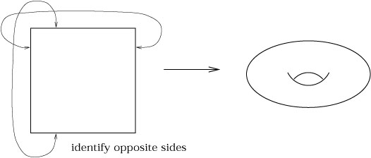
The notion of a manifold captures the idea of a space which may be
curved and have a complicated topology, but in local regions looks
just like
,
the set of n-tuples
(x1,..., xn).
The notion of a manifold captures the idea of a space which may be
curved and have a complicated topology, but in local regions looks
just like ![]() . (Here by "looks like" we do not mean that the
metric is the same, but only basic notions of analysis like open sets,
functions, and coordinates.) The entire manifold is constructed by
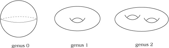
smoothly sewing together these local regions. Examples of manifolds
include:
. (Here by "looks like" we do not mean that the
metric is the same, but only basic notions of analysis like open sets,
functions, and coordinates.) The entire manifold is constructed by
smoothly sewing together these local regions. Examples of manifolds
include:
|
|
With all of these examples, the notion of a manifold may seem vacuous;
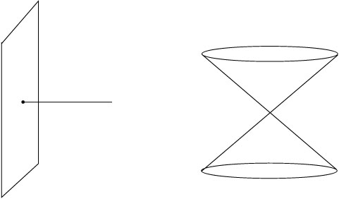
what isn't a manifold? There are plenty of things which are not
manifolds, because somewhere they do not look locally like ![]() .
Examples include a one-dimensional line running into a two-dimensional
plane, and two cones stuck together at their vertices. (A single cone
is okay; you can imagine smoothing out the vertex.)
.
Examples include a one-dimensional line running into a two-dimensional
plane, and two cones stuck together at their vertices. (A single cone
is okay; you can imagine smoothing out the vertex.)
|
We will now approach the rigorous definition of this simple idea, which requires a number of preliminary definitions. Many of them are pretty clear anyway, but it's nice to be complete.
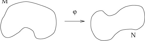
The most elementary notion is that of a map between two sets.
(We assume you know what a set is.) Given two sets M and N, a
map
![]() : M
: M ![]() N is a relationship which assigns, to each
element of M, exactly one element of N. A map is therefore
just a
simple generalization of a function. The canonical picture of a
map looks like this:
N is a relationship which assigns, to each
element of M, exactly one element of N. A map is therefore
just a
simple generalization of a function. The canonical picture of a
map looks like this:
|
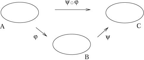
Given two maps
![]() : A
: A ![]() B and
B and
![]() : B
: B ![]() C,
we define the composition
C,
we define the composition
![]() o
o![]() : A
: A ![]() C
by the operation
(
C
by the operation
(![]() o
o![]() )(a) =
)(a) = ![]() (
(![]() (a)). So a
(a)). So a ![]() A,
A,
![]() (a)
(a) ![]() B, and thus
(
B, and thus
(![]() o
o![]() )(a)
)(a) ![]() C. The order in
which the maps are written makes sense, since the one on the right
acts first. In pictures:
C. The order in
which the maps are written makes sense, since the one on the right
acts first. In pictures:
|
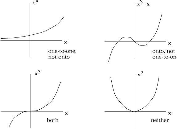
A map ![]() is called one-to-one (or "injective") if each
element of N has at most one element of M mapped into it, and
onto (or "surjective") if each element of N has at least one
element of M mapped into it. (If you think about it, a better
name for "one-to-one" would be "two-to-two".) Consider a function
is called one-to-one (or "injective") if each
element of N has at most one element of M mapped into it, and
onto (or "surjective") if each element of N has at least one
element of M mapped into it. (If you think about it, a better
name for "one-to-one" would be "two-to-two".) Consider a function
![]() :
: ![]()
![]()
![]() . Then
. Then
![]() (x) = ex is one-to-one, but not
onto;
(x) = ex is one-to-one, but not
onto;
![]() (x) = x3 - x is onto, but
not one-to-one;
(x) = x3 - x is onto, but
not one-to-one;
![]() (x) = x3 is both; and
(x) = x3 is both; and
![]() (x) = x2 is neither.
(x) = x2 is neither.
|
The set M is known as the domain
of the map ![]() , and the set of points in N which M gets
mapped into
is called the image of
, and the set of points in N which M gets
mapped into
is called the image of ![]() . For some subset
U
. For some subset
U ![]() N,
the set of elements of M which get mapped to U is called the
preimage of U under
N,
the set of elements of M which get mapped to U is called the
preimage of U under ![]() , or
, or
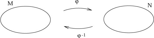
![]() (U). A map which
is both one-to-one and onto is known as invertible (or
"bijective"). In this case we can define the inverse map
(U). A map which
is both one-to-one and onto is known as invertible (or
"bijective"). In this case we can define the inverse map
![]() : N
: N ![]() M by
(
M by
(![]() o
o![]() )(a) = a. (Note that
the same symbol
)(a) = a. (Note that
the same symbol ![]() is used for both the preimage and the inverse
map, even though the former is always defined and the latter is
only defined in some special cases.) Thus:
is used for both the preimage and the inverse
map, even though the former is always defined and the latter is
only defined in some special cases.) Thus:
|
The notion of continuity of a map between topological spaces (and
thus manifolds) is actually a very subtle one, the precise formulation of
which we won't really
need. However the intuitive notions of continuity and differentiability
of maps
![]() :
: ![]()
![]()
![]() between Euclidean spaces are useful.
A map from
between Euclidean spaces are useful.
A map from ![]() to
to ![]() takes an m-tuple
(x1, x2,..., xm)
to an n-tuple
(y1, y2,..., yn),
and can therefore
be thought of as a collection of n functions
takes an m-tuple
(x1, x2,..., xm)
to an n-tuple
(y1, y2,..., yn),
and can therefore
be thought of as a collection of n functions ![]() of m variables:
of m variables:
| (2.1) |
We will refer to any one of these functions as Cp if
it is continuous
and p-times differentiable, and refer to the entire map
![]() :
: ![]()
![]()
![]() as Cp if each of its component
functions
are at least Cp. Thus a C0 map is
continuous but not necessarily differentiable,
while a C
as Cp if each of its component
functions
are at least Cp. Thus a C0 map is
continuous but not necessarily differentiable,
while a C![]() map is continuous and can be
differentiated as many times as you like. C
map is continuous and can be
differentiated as many times as you like. C![]() maps are sometimes called smooth.
We will call two sets M and N diffeomorphic if
there exists a C
maps are sometimes called smooth.
We will call two sets M and N diffeomorphic if
there exists a C![]() map
map
![]() : M
: M ![]() N with a C
N with a C![]() inverse
inverse
![]() : N
: N ![]() M; the map
M; the map ![]() is then called a diffeomorphism.
is then called a diffeomorphism.
Aside: The notion of two spaces being diffeomorphic only applies to
manifolds, where a notion of differentiability is inherited from the
fact that the space resembles ![]() locally. But "continuity" of maps
between topological spaces (not necessarily manifolds) can be defined,
and we say that two such spaces are "homeomorphic," which means
"topologically equivalent to," if there is a continuous map
between them with a continuous inverse. It is therefore conceivable that
spaces exist which are homeomorphic but not diffeomorphic; topologically
the same but with distinct "differentiable structures." In 1964 Milnor
showed that S7 had 28 different differentiable
structures;
it turns out that for n < 7 there is only one differentiable
structure on Sn, while for n > 7 the number
grows very large.
locally. But "continuity" of maps
between topological spaces (not necessarily manifolds) can be defined,
and we say that two such spaces are "homeomorphic," which means
"topologically equivalent to," if there is a continuous map
between them with a continuous inverse. It is therefore conceivable that
spaces exist which are homeomorphic but not diffeomorphic; topologically
the same but with distinct "differentiable structures." In 1964 Milnor
showed that S7 had 28 different differentiable
structures;
it turns out that for n < 7 there is only one differentiable
structure on Sn, while for n > 7 the number
grows very large.
![]() has infinitely many differentiable structures.
has infinitely many differentiable structures.
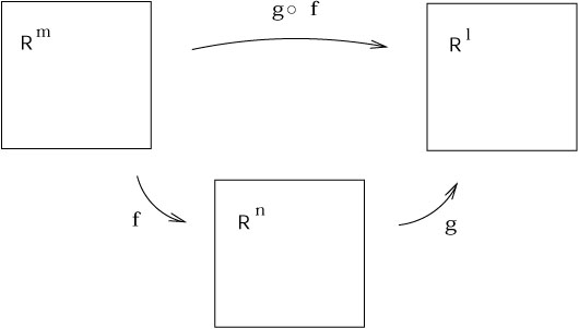
One piece of conventional calculus that we will need later is the
chain rule. Let us imagine that we have maps
f : ![]()
![]()
![]() and
g :
and
g : ![]()
![]()
![]() , and therefore the composition
(gof ):
, and therefore the composition
(gof ): ![]()
![]()
![]() .
.
|
We can represent each space in terms of coordinates:
xa on ![]() , yb on
, yb on ![]() , and zc on
, and zc on ![]() , where the
indices range over the appropriate values.
The chain rule relates the partial derivatives of the
composition to the partial derivatives of the individual maps:
, where the
indices range over the appropriate values.
The chain rule relates the partial derivatives of the
composition to the partial derivatives of the individual maps:
| (2.2) |
This is usually abbreviated to
| (2.3) |
There is nothing illegal or immoral about using this form of
the chain rule, but you should be able to visualize the maps that
underlie the construction. Recall that when m = n the
determinant of the matrix
![]() yb/
yb/![]() xa is called the Jacobian of the
map, and the map is invertible whenever the
Jacobian is nonzero.
xa is called the Jacobian of the
map, and the map is invertible whenever the
Jacobian is nonzero.
These basic definitions were presumably familiar to you, even if only vaguely remembered. We will now put them to use in the rigorous definition of a manifold. Unfortunately, a somewhat baroque procedure is required to formalize this relatively intuitive notion. We will first have to define the notion of an open set, on which we can put coordinate systems, and then sew the open sets together in an appropriate way.
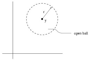
Start with the notion of an open ball, which is the set of all
points x in ![]() such that | x - y| < r
for some fixed
y
such that | x - y| < r
for some fixed
y ![]()
![]() and
r
and
r ![]()
![]() , where | x - y| = [
, where | x - y| = [![]() (xi -
yi)2]1/2. Note that this is
a strict inequality - the open ball is the interior of an n-sphere
of radius r centered at y.
(xi -
yi)2]1/2. Note that this is
a strict inequality - the open ball is the interior of an n-sphere
of radius r centered at y.
|
An open set in ![]() is a set constructed from an arbitrary
(maybe infinite) union of open balls. In other words,
V
is a set constructed from an arbitrary
(maybe infinite) union of open balls. In other words,
V ![]()
![]() is
open if, for any y
is
open if, for any y ![]() V, there is an open ball centered at y which
is completely inside V. Roughly speaking, an open set is the interior
of some (n - 1)-dimensional closed surface (or the union of
several such
interiors). By defining a notion of open sets, we have equipped
V, there is an open ball centered at y which
is completely inside V. Roughly speaking, an open set is the interior
of some (n - 1)-dimensional closed surface (or the union of
several such
interiors). By defining a notion of open sets, we have equipped ![]() with a topology - in this case, the "standard metric topology."
with a topology - in this case, the "standard metric topology."
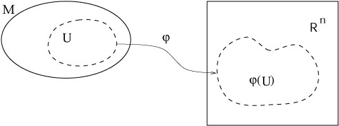
A chart or coordinate system consists of a subset U
of a set M, along with a one-to-one map
![]() : U
: U ![]()
![]() , such that the
image
, such that the
image ![]() (U) is open in
(U) is open in ![]() . (Any map is onto its image, so the map
. (Any map is onto its image, so the map
![]() : U
: U ![]()
![]() (U) is invertible.) We then can say that
U is an open set in M. (We have thus induced a topology on
M,
although we will not explore this.)
(U) is invertible.) We then can say that
U is an open set in M. (We have thus induced a topology on
M,
although we will not explore this.)
|
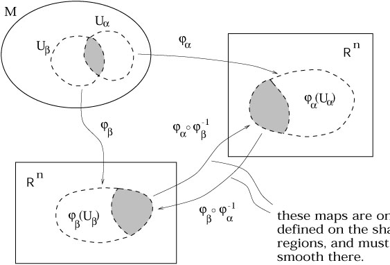
A C![]() atlas is an indexed collection
of charts
{(U
atlas is an indexed collection
of charts
{(U![]() ,
,![]() )} which satisfies two conditions:
)} which satisfies two conditions:
|
So a chart is what we normally think of as a coordinate system on some open set, and an atlas is a system of charts which are smoothly related on their overlaps.
At long last, then: a C![]() n-dimensional manifold
(or
n-manifold for short) is simply a set M along with a
"maximal atlas",
one that contains every possible compatible chart. (We can also replace
C
n-dimensional manifold
(or
n-manifold for short) is simply a set M along with a
"maximal atlas",
one that contains every possible compatible chart. (We can also replace
C![]() by Cp in all the
above definitions. For our purposes the degree
of differentiability of a manifold is not crucial; we will always assume
that any manifold is as differentiable as necessary for the application
under consideration.) The requirement that the
atlas be maximal is so that two equivalent spaces equipped with
different atlases don't count as different manifolds.
This definition captures in
formal terms our notion of a set that looks locally like
by Cp in all the
above definitions. For our purposes the degree
of differentiability of a manifold is not crucial; we will always assume
that any manifold is as differentiable as necessary for the application
under consideration.) The requirement that the
atlas be maximal is so that two equivalent spaces equipped with
different atlases don't count as different manifolds.
This definition captures in
formal terms our notion of a set that looks locally like ![]() .
Of course we will rarely have to make use of the full power of the
definition, but precision is its own reward.
.
Of course we will rarely have to make use of the full power of the
definition, but precision is its own reward.
One thing that is nice about our definition is that it does not rely
on an embedding of the manifold in some higher-dimensional Euclidean
space. In fact any n-dimensional manifold can be embedded in
![]() ("Whitney's embedding theorem"),
and sometimes we will make use of this fact (such as
in our definition of the sphere above). But it's important to
recognize that the manifold has an individual existence independent
of any embedding. We have no reason to believe, for example, that
four-dimensional spacetime is stuck in some larger space. (Actually
a number of people, string theorists and so forth, believe that our
four-dimensional world is part of a ten- or eleven-dimensional
spacetime, but as far as GR
is concerned the 4-dimensional view is perfectly adequate.)
("Whitney's embedding theorem"),
and sometimes we will make use of this fact (such as
in our definition of the sphere above). But it's important to
recognize that the manifold has an individual existence independent
of any embedding. We have no reason to believe, for example, that
four-dimensional spacetime is stuck in some larger space. (Actually
a number of people, string theorists and so forth, believe that our
four-dimensional world is part of a ten- or eleven-dimensional
spacetime, but as far as GR
is concerned the 4-dimensional view is perfectly adequate.)
Why was it necessary to be so finicky about charts and their overlaps,
rather than just covering every manifold with a single chart? Because
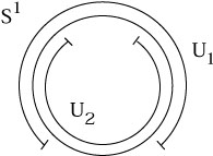
most manifolds cannot be covered with just one chart. Consider the
simplest example, S1. There is a conventional
coordinate system,
![]() : S1
: S1 ![]()
![]() , where
, where ![]() = 0 at the top of the circle
and wraps around to 2
= 0 at the top of the circle
and wraps around to 2![]() . However, in the definition of a chart we
have required that the image
. However, in the definition of a chart we
have required that the image
![]() (S1) be open in
(S1) be open in ![]() . If we
include either
. If we
include either ![]() = 0 or
= 0 or
![]() = 2
= 2![]() , we have a closed interval
rather than an open one; if we exclude both points, we haven't covered
the whole circle. So we need at least two charts, as shown.
, we have a closed interval
rather than an open one; if we exclude both points, we haven't covered
the whole circle. So we need at least two charts, as shown.
|
A somewhat more complicated example is provided by S2,
where once
again no single chart will cover the manifold. A Mercator projection,
traditionally used for world maps, misses both the North and South poles
(as well as the International Date Line, which involves the same problem
with ![]() that we found for S1.) Let's take
S2 to be the set
of points in
that we found for S1.) Let's take
S2 to be the set
of points in ![]() defined by
(x1)2 + (x2)2
+ (x3)2 = 1. We
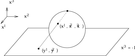
can construct a chart from an open set U1, defined to
be the sphere minus the north pole, via "stereographic projection":
defined by
(x1)2 + (x2)2
+ (x3)2 = 1. We
can construct a chart from an open set U1, defined to
be the sphere minus the north pole, via "stereographic projection":
|
Thus, we draw a straight line from the north pole to the plane defined by x3 = - 1, and assign to the point on S2 intercepted by the line the Cartesian coordinates (y1, y2) of the appropriate point on the plane. Explicitly, the map is given by
| (2.4) |
You are encouraged to check this for yourself. Another chart
(U2,![]() ) is obtained by projecting from the south pole to the
plane defined by x3 = + 1. The resulting coordinates
cover the sphere minus the south pole, and are given by
) is obtained by projecting from the south pole to the
plane defined by x3 = + 1. The resulting coordinates
cover the sphere minus the south pole, and are given by
| (2.5) |
Together, these two charts cover the entire manifold, and they overlap
in the region -1 < x3 < + 1. Another thing you can check is that the
composition
![]() o
o![]() is given by
is given by
| (2.6) |
and is C![]() in the region of overlap. As long as
we restrict
our attention to this region, (2.6) is just what we normally think
of as a change of coordinates.
in the region of overlap. As long as
we restrict
our attention to this region, (2.6) is just what we normally think
of as a change of coordinates.
We therefore see the necessity of charts and atlases: many manifolds
cannot be covered with a single coordinate system. (Although some
can, even ones with nontrivial topology. Can you think of a single
good coordinate system that covers the cylinder,
S1 × ![]() ?)
Nevertheless, it is very often most convenient to work with a single
chart, and just keep track of the set of points which aren't included.
?)
Nevertheless, it is very often most convenient to work with a single
chart, and just keep track of the set of points which aren't included.
The fact that manifolds look locally like ![]() , which is manifested
by the construction of coordinate charts, introduces the possibility
of analysis on manifolds, including operations such as differentiation
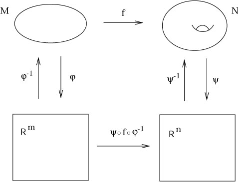
and integration. Consider two manifolds M and N of dimensions
m and n, with coordinate charts
, which is manifested
by the construction of coordinate charts, introduces the possibility
of analysis on manifolds, including operations such as differentiation
and integration. Consider two manifolds M and N of dimensions
m and n, with coordinate charts ![]() on M and
on M and ![]() on N.
Imagine we have a function
f : M
on N.
Imagine we have a function
f : M ![]() N,
N,
|
Just thinking of M and N as sets, we cannot nonchalantly
differentiate the map f, since we don't know what such an operation
means. But the coordinate charts allow us to construct the map
(![]() ofo
ofo![]() ) :
) : ![]()
![]()
![]() . (Feel free to
insert the words "where the maps are defined" wherever appropriate,
here and later on.) This is just
a map between Euclidean spaces, and all of the concepts of advanced
calculus apply. For example f, thought of as an N-valued
function on M, can be differentiated to obtain
. (Feel free to
insert the words "where the maps are defined" wherever appropriate,
here and later on.) This is just
a map between Euclidean spaces, and all of the concepts of advanced
calculus apply. For example f, thought of as an N-valued
function on M, can be differentiated to obtain
![]() f/
f/![]() x
x![]() , where the x
, where the x![]() represent
represent ![]() .
The point is that this notation is a shortcut, and what is really
going on is
.
The point is that this notation is a shortcut, and what is really
going on is
| (2.7) |
It would be far too unwieldy (not to mention pedantic) to write out the coordinate maps explicitly in every case. The shorthand notation of the left-hand-side will be sufficient for most purposes.
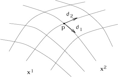
Having constructed this groundwork, we can now proceed to introduce various kinds of structure on manifolds. We begin with vectors and tangent spaces. In our discussion of special relativity we were intentionally vague about the definition of vectors and their relationship to the spacetime. One point that was stressed was the notion of a tangent space - the set of all vectors at a single point in spacetime. The reason for this emphasis was to remove from your minds the idea that a vector stretches from one point on the manifold to another, but instead is just an object associated with a single point. What is temporarily lost by adopting this view is a way to make sense of statements like "the vector points in the x direction" - if the tangent space is merely an abstract vector space associated with each point, it's hard to know what this should mean. Now it's time to fix the problem.
Let's imagine that we wanted to construct the tangent space at a
point p in a manifold M, using only things that are intrinsic
to M (no embeddings in higher-dimensional spaces etc.). One first
guess might be to use our intuitive knowledge that there are
objects called "tangent vectors to curves" which
belong in the tangent space. We might therefore consider the set
of all parameterized curves through p - that is,
the space of all (nondegenerate) maps
![]() :
: ![]()
![]() M such
that p is in the image of
M such
that p is in the image of ![]() . The temptation is to define
the tangent space as simply the space of all tangent vectors to
these curves at the point p. But this is obviously cheating; the
tangent space Tp is supposed to be the space of
vectors at p,
and before we have defined this we don't have an independent notion
of what "the tangent vector to a curve" is supposed to mean. In
some coordinate system x
. The temptation is to define
the tangent space as simply the space of all tangent vectors to
these curves at the point p. But this is obviously cheating; the
tangent space Tp is supposed to be the space of
vectors at p,
and before we have defined this we don't have an independent notion
of what "the tangent vector to a curve" is supposed to mean. In
some coordinate system x![]() any curve through p defines an
element of
any curve through p defines an
element of ![]() specified by the n real numbers
dx
specified by the n real numbers
dx![]() /d
/d![]() (where
(where ![]() is the parameter along the curve),
but this map is clearly coordinate-dependent, which is not what we
want.
is the parameter along the curve),
but this map is clearly coordinate-dependent, which is not what we
want.
Nevertheless we are on the right track, we just have to make things
independent of coordinates. To this end we define ![]() to be
the space of all smooth functions on M (that is, C
to be
the space of all smooth functions on M (that is, C![]() maps
f : M
maps
f : M ![]()
![]() ). Then we notice that each curve through p
defines an operator on this space, the directional derivative, which
maps
f
). Then we notice that each curve through p
defines an operator on this space, the directional derivative, which
maps
f ![]() df /d
df /d![]() (at p). We will make the following
claim: the tangent space Tp can be identified with
the space
of directional derivative operators along curves through p. To
establish this idea we must demonstrate two things: first, that the
space of directional derivatives is a vector space, and second that
it is the vector space we want (it has the same dimensionality as M,
yields a natural idea of a vector pointing along a certain direction,
and so on).
(at p). We will make the following
claim: the tangent space Tp can be identified with
the space
of directional derivative operators along curves through p. To
establish this idea we must demonstrate two things: first, that the
space of directional derivatives is a vector space, and second that
it is the vector space we want (it has the same dimensionality as M,
yields a natural idea of a vector pointing along a certain direction,
and so on).
The first claim, that directional derivatives form a vector space,
seems straightforward enough. Imagine two operators
![]() and
and
![]() representing derivatives along two curves
through p.
There is no problem adding these and scaling by real numbers, to
obtain a new operator
a
representing derivatives along two curves
through p.
There is no problem adding these and scaling by real numbers, to
obtain a new operator
a![]() + b
+ b![]() . It is
not immediately obvious, however, that the space closes; i.e.,
that the resulting operator is itself a derivative operator. A good
derivative operator is one that acts linearly on functions, and obeys
the conventional Leibniz (product) rule on products of functions.
Our new operator is manifestly linear, so we need to verify that it
obeys the Leibniz rule. We have
. It is
not immediately obvious, however, that the space closes; i.e.,
that the resulting operator is itself a derivative operator. A good
derivative operator is one that acts linearly on functions, and obeys
the conventional Leibniz (product) rule on products of functions.
Our new operator is manifestly linear, so we need to verify that it
obeys the Leibniz rule. We have
| (2.8) |
As we had hoped, the product rule is satisfied, and the set of directional derivatives is therefore a vector space.
Is it the vector space that we would like to identify with the tangent
space? The easiest way to become convinced is to find a basis for
the space. Consider again a coordinate chart with coordinates
x![]() .
Then there is an obvious set of n directional derivatives at
p,
namely the partial derivatives
.
Then there is an obvious set of n directional derivatives at
p,
namely the partial derivatives
![]() at p.
at p.
|
We are now going to claim that the partial derivative
operators
{![]() } at p form a basis for the tangent
space Tp.
(It follows immediately that Tp is
n-dimensional, since that is
the number of basis vectors.) To see this we will show that any
directional derivative can be decomposed into a sum of real numbers
times partial derivatives. This is in fact just the familiar
expression for the components of a tangent vector, but it's nice to
see it from the big-machinery approach. Consider an n-manifold
M, a coordinate chart
} at p form a basis for the tangent
space Tp.
(It follows immediately that Tp is
n-dimensional, since that is
the number of basis vectors.) To see this we will show that any
directional derivative can be decomposed into a sum of real numbers
times partial derivatives. This is in fact just the familiar
expression for the components of a tangent vector, but it's nice to
see it from the big-machinery approach. Consider an n-manifold
M, a coordinate chart
![]() : M
: M ![]()
![]() , a curve
, a curve
![]() :
: ![]()
![]() M, and a function
f : M
M, and a function
f : M ![]()
![]() .
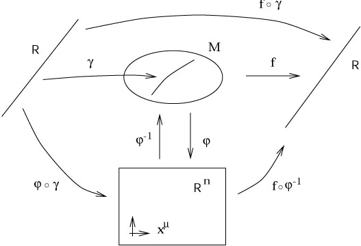
This leads to the following tangle of maps:
.
This leads to the following tangle of maps:
|
If ![]() is the parameter along
is the parameter along ![]() , we want to
expand the vector/operator
, we want to
expand the vector/operator
![]() in terms of the partials
in terms of the partials
![]() . Using the chain rule (2.2), we have
. Using the chain rule (2.2), we have
| (2.9) |
The first line simply takes the informal expression on the left hand
side and rewrites it as an honest derivative of the function
(fo![]() ) :
) : ![]()
![]()
![]() . The second line just comes from the
definition of the inverse map
. The second line just comes from the
definition of the inverse map ![]() (and associativity of the
operation of composition). The third line is the formal chain rule
(2.2), and the last line is a return to the informal notation of
the start. Since the function f was arbitrary, we have
(and associativity of the
operation of composition). The third line is the formal chain rule
(2.2), and the last line is a return to the informal notation of
the start. Since the function f was arbitrary, we have

| (2.10) |
Thus, the partials
{![]() } do indeed represent a good basis for the
vector space of directional derivatives, which we can therefore
safely identify with the tangent space.
} do indeed represent a good basis for the
vector space of directional derivatives, which we can therefore
safely identify with the tangent space.
Of course, the vector represented by
![]() is one
we already know; it's the tangent vector to the curve with parameter
is one
we already know; it's the tangent vector to the curve with parameter
![]() . Thus (2.10) can be thought of as a restatement of
(1.24),
where we claimed the that components of the tangent vector were
simply
dx
. Thus (2.10) can be thought of as a restatement of
(1.24),
where we claimed the that components of the tangent vector were
simply
dx![]() /d
/d![]() . The only difference is that we are working
on an arbitrary manifold, and we have specified our basis vectors
to be
. The only difference is that we are working
on an arbitrary manifold, and we have specified our basis vectors
to be
![]() =
= ![]() .
.
This particular basis (![]() =
= ![]() ) is known as a coordinate
basis for Tp; it is the formalization of the
notion of setting up
the basis vectors to point along the coordinate axes.
There is no reason why we are limited to coordinate
bases when we consider tangent vectors; it is sometimes more convenient,
for example, to use orthonormal bases of some sort. However, the
coordinate basis is very simple and natural, and we will use it
almost exclusively throughout the course.
) is known as a coordinate
basis for Tp; it is the formalization of the
notion of setting up
the basis vectors to point along the coordinate axes.
There is no reason why we are limited to coordinate
bases when we consider tangent vectors; it is sometimes more convenient,
for example, to use orthonormal bases of some sort. However, the
coordinate basis is very simple and natural, and we will use it
almost exclusively throughout the course.
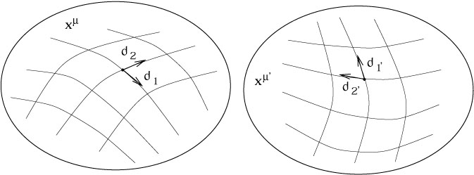
One of the advantages of the rather abstract point of view we have
taken toward vectors is that the transformation law is
immediate. Since the basis vectors are
![]() =
= ![]() , the basis
vectors in some new coordinate system x
, the basis
vectors in some new coordinate system x![]() are given by
the chain rule (2.3) as
are given by
the chain rule (2.3) as

| (2.11) |
We can get the transformation law for vector components by the same
technique used in flat space, demanding the the vector
V = V![]()
![]() be unchanged by a change of basis. We have
be unchanged by a change of basis. We have
| (2.12) |
and hence (since the matrix
![]() x
x![]() /
/![]() x
x![]() is the
inverse of the matrix
is the
inverse of the matrix
![]() x
x![]() /
/![]() x
x![]() ),
),

| (2.13) |
Since the basis vectors are usually not written explicitly, the rule
(2.13) for transforming components is what we call the "vector
transformation law." We notice that it is compatible with the
transformation of vector components in special relativity under
Lorentz transformations, V![]() =
= ![]()
![]() V
V![]() ,
since a Lorentz transformation is a special kind of coordinate
transformation, with
x
,
since a Lorentz transformation is a special kind of coordinate
transformation, with
x![]() =
= ![]()
![]() x
x![]() . But
(2.13) is much more general, as it encompasses the behavior of vectors
under arbitrary changes of coordinates (and therefore bases), not just
linear transformations. As usual, we are trying to emphasize a
somewhat subtle ontological distinction - tensor components do not
change when we change coordinates, they change when we change the
basis in the tangent space, but we have decided to use the coordinates
to define our basis. Therefore a change of coordinates induces a
change of basis:
. But
(2.13) is much more general, as it encompasses the behavior of vectors
under arbitrary changes of coordinates (and therefore bases), not just
linear transformations. As usual, we are trying to emphasize a
somewhat subtle ontological distinction - tensor components do not
change when we change coordinates, they change when we change the
basis in the tangent space, but we have decided to use the coordinates
to define our basis. Therefore a change of coordinates induces a
change of basis:
|
Having explored the world of vectors, we continue to retrace the steps
we took in flat space, and now consider dual vectors (one-forms).
Once again the cotangent space T*p is the
set of linear maps
![]() : Tp
: Tp ![]()
![]() . The canonical example of a one-form is
the gradient of a function f, denoted df. Its action on a
vector
. The canonical example of a one-form is
the gradient of a function f, denoted df. Its action on a
vector
![]() is exactly the directional derivative of
the function:
is exactly the directional derivative of
the function:
| (2.14) |
It's tempting to think, "why shouldn't the function f itself be
considered the one-form, and df /d![]() its action?" The point
is that a one-form, like a vector, exists only at the point it
is defined, and does not depend on information at other points on M.
If you know a function in some neighborhood of a point you can take
its derivative, but not just from knowing its value at the point;
the gradient, on the other hand, encodes precisely the
information necessary to take the directional derivative along any curve
through p, fulfilling its role as a dual vector.
its action?" The point
is that a one-form, like a vector, exists only at the point it
is defined, and does not depend on information at other points on M.
If you know a function in some neighborhood of a point you can take
its derivative, but not just from knowing its value at the point;
the gradient, on the other hand, encodes precisely the
information necessary to take the directional derivative along any curve
through p, fulfilling its role as a dual vector.
Just as the partial derivatives along coordinate axes provide a natural
basis for the tangent space, the gradients of the coordinate functions
x![]() provide a natural basis for the
cotangent space. Recall that in
flat space we constructed a basis for T*p
by demanding that
provide a natural basis for the
cotangent space. Recall that in
flat space we constructed a basis for T*p
by demanding that
![]() (
(![]() ) =
) = ![]() . Continuing the same philosophy on an
arbitrary manifold, we find that (2.14) leads to
. Continuing the same philosophy on an
arbitrary manifold, we find that (2.14) leads to
| (2.15) |
Therefore the gradients
{dx![]() } are an appropriate set of
basis one-forms; an arbitrary one-form is expanded into components
as
} are an appropriate set of
basis one-forms; an arbitrary one-form is expanded into components
as
![]() =
= ![]() dx
dx![]() .
.
The transformation properties of basis dual vectors and components follow from what is by now the usual procedure. We obtain, for basis one-forms,
| (2.16) |
and for components,

| (2.17) |
We will usually write the components
![]() when we speak about a
one-form
when we speak about a
one-form ![]() .
.
The transformation law for general tensors follows this same pattern of replacing the Lorentz transformation matrix used in flat space with a matrix representing more general coordinate transformations. A (k, l ) tensor T can be expanded

| (2.18) |
and under a coordinate transformation the components change according to
| (2.19) |
This tensor transformation law is straightforward to remember, since there really isn't anything else it could be, given the placement of indices. However, it is often easier to transform a tensor by taking the identity of basis vectors and one-forms as partial derivatives and gradients at face value, and simply substituting in the coordinate transformation. As an example consider a symmetric (0, 2) tensor S on a 2-dimensional manifold, whose components in a coordinate system (x1 = x, x2 = y) are given by
| (2.20) |
This can be written equivalently as
| (2.21) |
where in the last line the tensor product symbols are suppressed for brevity. Now consider new coordinates

| (2.22) |
This leads directly to
| (2.23) |
We need only plug these expressions directly into (2.21) to obtain
(remembering that tensor products don't commute, so
dx' dy' ![]() dy' dx'):
dy' dx'):

| (2.24) |
or
| (2.25) |
Notice that it is still symmetric. We did not use the transformation law (2.19) directly, but doing so would have yielded the same result, as you can check.
For the most part the various tensor operations we defined in flat space are unaltered in a more general setting: contraction, symmetrization, etc. There are three important exceptions: partial derivatives, the metric, and the Levi-Civita tensor. Let's look at the partial derivative first.
The unfortunate fact is that the partial derivative of a tensor is
not, in general, a new tensor. The gradient, which is the partial
derivative of a scalar, is an honest (0, 1) tensor, as we have
seen. But the partial derivative of higher-rank tensors is not
tensorial, as we can see by considering
the partial derivative of a one-form,
![]() W
W![]() , and changing to
a new coordinate system:
, and changing to
a new coordinate system:
| (2.26) |
The second term in the last line should not be there if
![]() W
W![]() were to transform as a (0, 2) tensor. As you can see, it arises because
the derivative of the transformation matrix does not vanish, as it did
for Lorentz transformations in flat space.
were to transform as a (0, 2) tensor. As you can see, it arises because
the derivative of the transformation matrix does not vanish, as it did
for Lorentz transformations in flat space.
On the other hand, the exterior derivative operator d does form an antisymmetric (0, p + 1) tensor when acted on a p-form. For p = 1 we can see this from (2.26); the offending non-tensorial term can be written
| (2.27) |
This expression is symmetric in ![]() and
and ![]() , since partial
derivatives commute. But the exterior derivative is defined to be
the antisymmetrized partial derivative, so this term vanishes (the
antisymmetric part of a symmetric expression is zero). We are then
left with the correct tensor transformation law; extension to arbitrary
p is straightforward. So the exterior derivative is a legitimate
tensor operator; it is not, however, an adequate substitute for the
partial derivative, since it is only defined on forms. In the next
section we will define a covariant derivative, which can be thought
of as the extension of the partial derivative to arbitrary manifolds.
, since partial
derivatives commute. But the exterior derivative is defined to be
the antisymmetrized partial derivative, so this term vanishes (the
antisymmetric part of a symmetric expression is zero). We are then
left with the correct tensor transformation law; extension to arbitrary
p is straightforward. So the exterior derivative is a legitimate
tensor operator; it is not, however, an adequate substitute for the
partial derivative, since it is only defined on forms. In the next
section we will define a covariant derivative, which can be thought
of as the extension of the partial derivative to arbitrary manifolds.
The metric tensor is such an important object in curved space that
it is given a new symbol,
g![]()
![]() (while
(while
![]() is reserved
specifically for the Minkowski metric). There are few restrictions
on the components of
g
is reserved
specifically for the Minkowski metric). There are few restrictions
on the components of
g![]()
![]() , other than that it be a symmetric
(0, 2) tensor. It is usually taken to be non-degenerate, meaning that
the determinant
g = | g
, other than that it be a symmetric
(0, 2) tensor. It is usually taken to be non-degenerate, meaning that
the determinant
g = | g![]()
![]() | doesn't vanish. This allows us to define
the inverse metric
g
| doesn't vanish. This allows us to define
the inverse metric
g![]()
![]() via
via

| (2.28) |
The symmetry of g![]()
![]() implies that
g
implies that
g![]()
![]() is also symmetric.
Just as in special relativity, the metric and its inverse may be
used to raise and lower indices on tensors.
is also symmetric.
Just as in special relativity, the metric and its inverse may be
used to raise and lower indices on tensors.
It will take several weeks to fully appreciate the role of the
metric in all of its glory, but for purposes of inspiration we can
list the various uses to which
g![]()
![]() will be put: (1) the metric
supplies a notion of "past" and "future"; (2) the metric
allows the computation of path length and proper time; (3) the metric
determines the "shortest distance" between two points (and therefore
the motion of test particles); (4) the metric replaces the Newtonian
gravitational field
will be put: (1) the metric
supplies a notion of "past" and "future"; (2) the metric
allows the computation of path length and proper time; (3) the metric
determines the "shortest distance" between two points (and therefore
the motion of test particles); (4) the metric replaces the Newtonian
gravitational field ![]() ; (5) the metric provides a notion of
locally inertial frames and therefore a sense of "no rotation";
(6) the metric determines causality, by defining the speed of light
faster than which no signal can travel; (7) the metric replaces the
traditional Euclidean three-dimensional dot product of Newtonian
mechanics; and so on. Obviously these ideas are not all completely
independent, but we get some sense of the importance of this tensor.
; (5) the metric provides a notion of
locally inertial frames and therefore a sense of "no rotation";
(6) the metric determines causality, by defining the speed of light
faster than which no signal can travel; (7) the metric replaces the
traditional Euclidean three-dimensional dot product of Newtonian
mechanics; and so on. Obviously these ideas are not all completely
independent, but we get some sense of the importance of this tensor.
In our discussion of path lengths in special relativity we (somewhat
handwavingly) introduced the line element as
ds2 = ![]() dx
dx![]() dx
dx![]() , which was used to get the length of a
path. Of course now that we know that
dx
, which was used to get the length of a
path. Of course now that we know that
dx![]() is really a basis dual vector, it
becomes natural to use the terms "metric" and "line element"
interchangeably, and write
is really a basis dual vector, it
becomes natural to use the terms "metric" and "line element"
interchangeably, and write
| (2.29) |
(To be perfectly consistent we should write this as "g", and
sometimes
will, but more often than not g is used for the determinant
| g![]()
![]() |.)
For example, we know that the Euclidean line element in a
three-dimensional space with Cartesian coordinates is
|.)
For example, we know that the Euclidean line element in a
three-dimensional space with Cartesian coordinates is
| (2.30) |
We can now change to any coordinate system we choose. For example, in spherical coordinates we have
| (2.31) |
which leads directly to

| (2.32) |
Obviously the components of the metric look different than those in Cartesian coordinates, but all of the properties of the space remain unaltered.
Perhaps this is a good time to note that most references are not
sufficiently picky to distinguish between
"dx", the informal notion of an infinitesimal displacement, and
"dx", the rigorous notion of a basis one-form given by the
gradient of a coordinate function. In fact our notation
"ds2"
does not refer to the exterior derivative of anything, or the square
of anything; it's just conventional shorthand for the metric tensor.
On the other hand, "(dx)2" refers specifically to the
(0, 2) tensor dx ![]() dx.
dx.
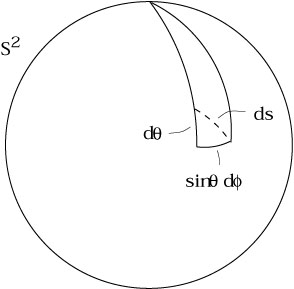
A good example of a
space with curvature is the two-sphere, which can be thought of
as the locus of points in ![]() at distance 1 from the origin. The
metric in the (
at distance 1 from the origin. The
metric in the (![]() ,
,![]() ) coordinate system comes from setting r = 1
and dr = 0 in (2.32):
) coordinate system comes from setting r = 1
and dr = 0 in (2.32):
| (2.33) |
This is completely consistent with the interpretation of ds as an infinitesimal length, as illustrated in the figure.
|
As we shall see, the metric tensor contains all the information we need
to describe the curvature of the manifold (at least in Riemannian
geometry; we will actually indicate somewhat more general approaches).
In Minkowski space we can choose coordinates in which the components of
the metric are constant; but it should be clear that the existence of
curvature is more subtle than having the metric depend on the coordinates,
since in the example above we showed how the metric in flat Euclidean
space in spherical coordinates is a function of r and ![]() . Later,
we shall see that constancy of the metric components is sufficient
for a space to be flat, and in fact there always exists a coordinate
system on any flat space in which the metric is constant. But we might
not want to work in such a coordinate system, and we might not even
know how to find it; therefore we will want a more precise characterization
of the curvature, which will be introduced down the road.
. Later,
we shall see that constancy of the metric components is sufficient
for a space to be flat, and in fact there always exists a coordinate
system on any flat space in which the metric is constant. But we might
not want to work in such a coordinate system, and we might not even
know how to find it; therefore we will want a more precise characterization
of the curvature, which will be introduced down the road.
A useful characterization of the metric is obtained by putting
g![]()
![]() into its canonical form. In this form the metric components
become
into its canonical form. In this form the metric components
become

| (2.34) |
where "diag" means a diagonal matrix with the given elements. If n is the dimension of the manifold, s is the number of +1's in the canonical form, and t is the number of -1's, then s - t is the signature of the metric (the difference in the number of minus and plus signs), and s + t is the rank of the metric (the number of nonzero eigenvalues). If a metric is continuous, the rank and signature of the metric tensor field are the same at every point, and if the metric is nondegenerate the rank is equal to the dimension n. We will always deal with continuous, nondegenerate metrics. If all of the signs are positive (t = 0) the metric is called Euclidean or Riemannian (or just "positive definite"), while if there is a single minus (t = 1) it is called Lorentzian or pseudo-Riemannian, and any metric with some +1's and some -1's is called "indefinite." (So the word "Euclidean" sometimes means that the space is flat, and sometimes doesn't, but always means that the canonical form is strictly positive; the terminology is unfortunate but standard.) The spacetimes of interest in general relativity have Lorentzian metrics.
We haven't yet demonstrated that it is always possible to but the metric
into canonical form. In fact it is always
possible to do so at some point p ![]() M, but in general it will only
be possible at that single point, not in any neighborhood of p.
Actually we can do slightly better than this; it turns out that at
any point p there exists a coordinate system in which
g
M, but in general it will only
be possible at that single point, not in any neighborhood of p.
Actually we can do slightly better than this; it turns out that at
any point p there exists a coordinate system in which
g![]()
![]() takes
its canonical form and the first derivatives
takes
its canonical form and the first derivatives
![]() g
g![]()
![]() all vanish
(while the second derivatives
all vanish
(while the second derivatives
![]()
![]() g
g![]()
![]() cannot be made
to all vanish). Such coordinates are known as Riemann normal
coordinates, and the associated basis vectors constitute
a local Lorentz frame. Notice
that in Riemann normal coordinates (or RNC's) the metric at p looks
like that of flat space "to first order." This is the rigorous
notion of the idea that "small enough regions of spacetime look like
flat (Minkowski) space." (Also, there is no difficulty in simultaneously
constructing sets of basis vectors at every point in M such that the
metric takes its canonical form; the problem is that in general this
will not be a coordinate basis, and there will be no way to
make it into one.)
cannot be made
to all vanish). Such coordinates are known as Riemann normal
coordinates, and the associated basis vectors constitute
a local Lorentz frame. Notice
that in Riemann normal coordinates (or RNC's) the metric at p looks
like that of flat space "to first order." This is the rigorous
notion of the idea that "small enough regions of spacetime look like
flat (Minkowski) space." (Also, there is no difficulty in simultaneously
constructing sets of basis vectors at every point in M such that the
metric takes its canonical form; the problem is that in general this
will not be a coordinate basis, and there will be no way to
make it into one.)
We won't consider the detailed proof of this statement; it can be found in Schutz, pp. 158-160, where it goes by the name of the "local flatness theorem." (He also calls local Lorentz frames "momentarily comoving reference frames," or MCRF's.) It is useful to see a sketch of the proof, however, for the specific case of a Lorentzian metric in four dimensions. The idea is to consider the transformation law for the metric
| (2.35) |
and expand both sides in Taylor series in the sought-after
coordinates x![]() . The expansion of the old
coordinates x
. The expansion of the old
coordinates x![]() looks like
looks like

| (2.36) |
with the other expansions proceeding along the same lines. (For
simplicity we have set
x![]() (p) = x
(p) = x![]() (p) = 0.) Then, using some
extremely schematic notation, the expansion of (2.35) to second order is
(p) = 0.) Then, using some
extremely schematic notation, the expansion of (2.35) to second order is
| (2.37) |
We can set terms of equal order in x' on each side equal to each
other. Therefore, the components
g![]()
![]() (p), 10 numbers in all (to
describe a symmetric two-index tensor), are determined by the
matrix
(
(p), 10 numbers in all (to
describe a symmetric two-index tensor), are determined by the
matrix
(![]() x
x![]() /
/![]() x
x![]() )p. This is a 4 × 4
matrix with no constraints; thus, 16 numbers we are free to choose.
Clearly this is enough freedom to put the 10 numbers of
g
)p. This is a 4 × 4
matrix with no constraints; thus, 16 numbers we are free to choose.
Clearly this is enough freedom to put the 10 numbers of
g![]()
![]() (p)
into canonical form, at least as far as having enough degrees of
freedom is concerned. (In fact there are some limitations - if you go
through the procedure carefully, you find for example that you cannot
change the signature and rank.) The six remaining degrees of freedom can
be interpreted as exactly the six parameters of the Lorentz group;
we know that these leave the canonical form unchanged. At first
order we have the derivatives
(p)
into canonical form, at least as far as having enough degrees of
freedom is concerned. (In fact there are some limitations - if you go
through the procedure carefully, you find for example that you cannot
change the signature and rank.) The six remaining degrees of freedom can
be interpreted as exactly the six parameters of the Lorentz group;
we know that these leave the canonical form unchanged. At first
order we have the derivatives
![]() g
g![]()
![]() (p), four
derivatives of ten components for a total of 40 numbers. But looking
at the right hand side of (2.37) we see that we now have the additional
freedom to choose
(
(p), four
derivatives of ten components for a total of 40 numbers. But looking
at the right hand side of (2.37) we see that we now have the additional
freedom to choose
(![]() x
x![]() /
/![]() x
x![]()
![]() x
x![]() )p. In this set
of numbers there are 10
independent choices of the indices
)p. In this set
of numbers there are 10
independent choices of the indices ![]() and
and ![]() (it's symmetric,
since partial derivatives commute) and four choices of
(it's symmetric,
since partial derivatives commute) and four choices of ![]() , for
a total of 40 degrees of freedom. This is precisely the amount of
choice we need to determine all of the first derivatives of the metric,
which we can therefore set to zero. At second order, however, we are
concerned with
, for
a total of 40 degrees of freedom. This is precisely the amount of
choice we need to determine all of the first derivatives of the metric,
which we can therefore set to zero. At second order, however, we are
concerned with
![]()
![]() g
g![]()
![]() (p); this is symmetric
in
(p); this is symmetric
in ![]() and
and ![]() as well as
as well as ![]() and
and ![]() , for a total of
10 × 10 = 100 numbers. Our ability to make additional choices
is contained in
(
, for a total of
10 × 10 = 100 numbers. Our ability to make additional choices
is contained in
(![]() x
x![]() /
/![]() x
x![]()
![]() x
x![]()
![]() x
x![]() )p. This is
symmetric in the three lower indices,
which gives 20 possibilities, times four for the upper index gives us
80 degrees of freedom - 20 fewer than we require to set the second
derivatives of the metric to zero. So in fact we cannot make the second
derivatives vanish; the deviation from flatness must therefore be
measured by the 20 coordinate-independent degrees of freedom representing
the second derivatives of the
metric tensor field. We will see later how this comes about, when we
characterize curvature using the Riemann tensor, which will turn out
to have 20 independent components.
)p. This is
symmetric in the three lower indices,
which gives 20 possibilities, times four for the upper index gives us
80 degrees of freedom - 20 fewer than we require to set the second
derivatives of the metric to zero. So in fact we cannot make the second
derivatives vanish; the deviation from flatness must therefore be
measured by the 20 coordinate-independent degrees of freedom representing
the second derivatives of the
metric tensor field. We will see later how this comes about, when we
characterize curvature using the Riemann tensor, which will turn out
to have 20 independent components.
The final change we have to make to our tensor knowledge now that
we have dropped the assumption of flat space has to do with the
Levi-Civita tensor,
![]() . Remember
that the flat-space version of this object, which we will now
denote by
. Remember
that the flat-space version of this object, which we will now
denote by
![]() , was defined
as
, was defined
as
| (2.38) |
We will now define the Levi-Civita symbol to be exactly this
![]() - that is, an object
with n indices which has the components specified above in
any coordinate system. This is called a "symbol," of course,
because it is not a tensor; it is defined not to change under
coordinate transformations. We can relate its behavior to that of
an ordinary tensor by first noting that, given some n ×
n matrix M
- that is, an object
with n indices which has the components specified above in
any coordinate system. This is called a "symbol," of course,
because it is not a tensor; it is defined not to change under
coordinate transformations. We can relate its behavior to that of
an ordinary tensor by first noting that, given some n ×
n matrix M![]()
![]() , the determinant | M|
obeys
, the determinant | M|
obeys

| (2.39) |
This is just a true fact about the determinant which you can find in
a sufficiently enlightened linear algebra book. If follows that,
setting
M![]()
![]() =
= ![]() x
x![]() /
/![]() x
x![]() , we have
, we have
| (2.40) |
This is close to the tensor transformation law, except for the
determinant out front. Objects which transform in this way are
known as tensor densities. Another example is given by
the determinant of the metric,
g = | g![]()
![]() |. It's easy to check
(by taking the determinant of both sides of (2.35)) that under a
coordinate transformation we get
|. It's easy to check
(by taking the determinant of both sides of (2.35)) that under a
coordinate transformation we get
| (2.41) |
Therefore g is also not a tensor; it transforms in a way similar to the Levi-Civita symbol, except that the Jacobian is raised to the -2 power. The power to which the Jacobian is raised is known as the weight of the tensor density; the Levi-Civita symbol is a density of weight 1, while g is a (scalar) density of weight -2.
However, we don't like tensor densities, we like tensors. There is a simple way to convert a density into an honest tensor - multiply by | g|w/2, where w is the weight of the density (the absolute value signs are there because g < 0 for Lorentz metrics). The result will transform according to the tensor transformation law. Therefore, for example, we can define the Levi-Civita tensor as
| (2.42) |
It is this tensor
which is used in the definition of the Hodge dual, (1.87), which
is otherwise unchanged when generalized to arbitrary manifolds.
Since this is a real tensor, we can raise indices, etc. Sometimes
people define a version of the Levi-Civita symbol with upper indices,
![]() , whose components are
numerically equal to the symbol with lower indices. This turns out
to be a density of weight -1, and is related to the tensor with
upper indices by
, whose components are
numerically equal to the symbol with lower indices. This turns out
to be a density of weight -1, and is related to the tensor with
upper indices by
| (2.43) |
As an aside, we should come clean and admit that, even with the factor
of ![]() , the Levi-Civita tensor is in some sense
not a true
tensor, because on some manifolds it cannot be globally defined. Those
on which it can be defined are called orientable, and we will deal
exclusively with orientable manifolds in this course. An example of
a non-orientable manifold is the Möbius strip; see Schutz's
Geometrical Methods in Mathematical Physics (or a similar text)
for a discussion.
, the Levi-Civita tensor is in some sense
not a true
tensor, because on some manifolds it cannot be globally defined. Those
on which it can be defined are called orientable, and we will deal
exclusively with orientable manifolds in this course. An example of
a non-orientable manifold is the Möbius strip; see Schutz's
Geometrical Methods in Mathematical Physics (or a similar text)
for a discussion.
One final appearance of tensor densities is in integration on manifolds.
We will not do this subject justice, but at least a casual glance is
necessary. You have probably been exposed to the fact that in ordinary
calculus on ![]() the volume
element dnx picks up a factor of the Jacobian under
change of coordinates:
the volume
element dnx picks up a factor of the Jacobian under
change of coordinates:
| (2.44) |
There is actually a beautiful explanation of this formula from the point of view of differential forms, which arises from the following fact: on an n-dimensional manifold, the integrand is properly understood as an n-form. The naive volume element dnx is itself a density rather than an n-form, but there is no difficulty in using it to construct a real n-form. To see how this works, we should make the identification
| (2.45) |
The expression on the right hand side can be misleading, because it looks
like a tensor (an n-form, actually) but is really a density.
Certainly if we have two
functions f and g on M, then df and
dg are one-forms, and
df ![]() dg is a two-form. But we would like to interpret
the right hand side of (2.45) as a coordinate-dependent object which,
in the x
dg is a two-form. But we would like to interpret
the right hand side of (2.45) as a coordinate-dependent object which,
in the x![]() coordinate system, acts like
dx0
coordinate system, acts like
dx0 ![]() ...
... ![]() dxn - 1. This sounds tricky, but in
fact it's just an
ambiguity of notation, and in practice we will just use the
shorthand notation "dnx".
dxn - 1. This sounds tricky, but in
fact it's just an
ambiguity of notation, and in practice we will just use the
shorthand notation "dnx".
To justify this song and dance, let's see how (2.45) changes under coordinate transformations. First notice that the definition of the wedge product allows us to write
| (2.46) |
since both the wedge product and the Levi-Civita symbol are completely
antisymmetric. Under a coordinate transformation
![]() stays the same while
the one-forms change according to (2.16), leading to
stays the same while
the one-forms change according to (2.16), leading to
| (2.47) |
Multiplying by the Jacobian on both sides recovers (2.44).
It is clear that the naive volume element dnx
transforms as a
density, not a tensor, but it is straightforward to construct an
invariant volume element by multiplying by
![]() :
:

| (2.48) |
which is of course just
(n!)-1![]() dx
dx![]()
![]() ...
... ![]() dx
dx![]() .
In the interest of simplicity we will usually write the volume
element as
.
In the interest of simplicity we will usually write the volume
element as
![]() dnx, rather than
as the explicit wedge product
dnx, rather than
as the explicit wedge product
![]() dx0
dx0 ![]() ...
... ![]() dxn - 1; it will
be enough to keep in mind that it's supposed to be an n-form.
dxn - 1; it will
be enough to keep in mind that it's supposed to be an n-form.
As a final aside to finish this section, let's consider one of the
most elegant and powerful theorems of differential geometry: Stokes's
theorem. This theorem is the generalization of the fundamental
theorem of calculus,
![]() dx = a - b. Imagine that we
have an n-manifold M with boundary
dx = a - b. Imagine that we
have an n-manifold M with boundary
![]() M, and an (n - 1)-form
M, and an (n - 1)-form
![]() on M. (We haven't discussed manifolds with
boundaries,
but the idea is obvious; M could for instance be the interior of
an (n - 1)-dimensional closed surface
on M. (We haven't discussed manifolds with
boundaries,
but the idea is obvious; M could for instance be the interior of
an (n - 1)-dimensional closed surface
![]() M.) Then
d
M.) Then
d![]() is an n-form, which can be integrated over M, while
is an n-form, which can be integrated over M, while ![]() itself
can be integrated over
itself
can be integrated over
![]() M. Stokes's theorem is then
M. Stokes's theorem is then
| (2.49) |
You can convince yourself that different special cases of this theorem include not only the fundamental theorem of calculus, but also the theorems of Green, Gauss, and Stokes, familiar from vector calculus in three dimensions.