


We will begin with a whirlwind tour of special relativity (SR) and life in flat spacetime. The point will be both to recall what SR is all about, and to introduce tensors and related concepts that will be crucial later on, without the extra complications of curvature on top of everything else. Therefore, for this section we will always be working in flat spacetime, and furthermore we will only use orthonormal (Cartesian-like) coordinates. Needless to say it is possible to do SR in any coordinate system you like, but it turns out that introducing the necessary tools for doing so would take us halfway to curved spaces anyway, so we will put that off for a while.
It is often said that special relativity is a theory of 4-dimensional spacetime: three of space, one of time. But of course, the pre-SR world of Newtonian mechanics featured three spatial dimensions and a time parameter. Nevertheless, there was not much temptation to consider these as different aspects of a single 4-dimensional spacetime. Why not?
|
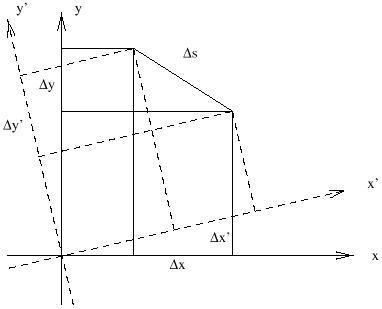
Consider a garden-variety 2-dimensional plane. It is typically convenient to label the points on such a plane by introducing coordinates, for example by defining orthogonal x and y axes and projecting each point onto these axes in the usual way. However, it is clear that most of the interesting geometrical facts about the plane are independent of our choice of coordinates. As a simple example, we can consider the distance between two points, given by
| (1.1) |
In a different Cartesian coordinate system, defined by x' and y' axes which are rotated with respect to the originals, the formula for the distance is unaltered:
| (1.2) |
We therefore say that the distance is invariant under such changes of coordinates.
|
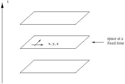
This is why it is useful to think of the plane as 2-dimensional: although we use two distinct numbers to label each point, the numbers are not the essence of the geometry, since we can rotate axes into each other while leaving distances and so forth unchanged. In Newtonian physics this is not the case with space and time; there is no useful notion of rotating space and time into each other. Rather, the notion of "all of space at a single moment in time" has a meaning independent of coordinates.
Such is not the case in SR. Let us consider coordinates (t, x, y, z) on spacetime, set up in the following way. The spatial coordinates (x, y, z) comprise a standard Cartesian system, constructed for example by welding together rigid rods which meet at right angles. The rods must be moving freely, unaccelerated. The time coordinate is defined by a set of clocks which are not moving with respect to the spatial coordinates. (Since this is a thought experiment, we imagine that the rods are infinitely long and there is one clock at every point in space.) The clocks are synchronized in the following sense: if you travel from one point in space to any other in a straight line at constant speed, the time difference between the clocks at the ends of your journey is the same as if you had made the same trip, at the same speed, in the other direction. The coordinate system thus constructed is an inertial frame.
An event is defined as a single moment in space and time, characterized uniquely by (t, x, y, z). Then, without any motivation for the moment, let us introduce the spacetime interval between two events:

| (1.3) |
(Notice that it can be positive, negative, or zero even for two nonidentical points.) Here, c is some fixed conversion factor between space and time; that is, a fixed velocity. Of course it will turn out to be the speed of light; the important thing, however, is not that photons happen to travel at that speed, but that there exists a c such that the spacetime interval is invariant under changes of coordinates. In other words, if we set up a new inertial frame (t', x', y', z') by repeating our earlier procedure, but allowing for an offset in initial position, angle, and velocity between the new rods and the old, the interval is unchanged:

| (1.4) |
This is why it makes sense to think of SR as a theory of 4-dimensional spacetime, known as Minkowski space. (This is a special case of a 4-dimensional manifold, which we will deal with in detail later.) As we shall see, the coordinate transformations which we have implicitly defined do, in a sense, rotate space and time into each other. There is no absolute notion of "simultaneous events"; whether two things occur at the same time depends on the coordinates used. Therefore the division of Minkowski space into space and time is a choice we make for our own purposes, not something intrinsic to the situation.
Almost all of the "paradoxes" associated with SR result from a stubborn persistence of the Newtonian notions of a unique time coordinate and the existence of "space at a single moment in time." By thinking in terms of spacetime rather than space and time together, these paradoxes tend to disappear.
Let's introduce some convenient notation. Coordinates on spacetime will be denoted by letters with Greek superscript indices running from 0 to 3, with 0 generally denoting the time coordinate. Thus,
| (1.5) |
(Don't start thinking of the superscripts as exponents.) Furthermore, for the sake of simplicity we will choose units in which

| (1.6) |
we will therefore leave out factors of c in all subsequent formulae.
Empirically we know that c is the speed of light,
3 × 10⁸ meters
per second; thus, we are working in units where 1 second equals
3 × 10⁸
meters. Sometimes it will be useful to refer to the space and time
components of x![]() separately, so we will use Latin
superscripts to
stand for the space components alone:
separately, so we will use Latin
superscripts to
stand for the space components alone:
| (1.7) |
It is also convenient to write the spacetime interval in a more compact form. We therefore introduce a 4 × 4 matrix, the metric, which we write using two lower indices:
| (1.8) |
(Some references, especially field theory books, define the metric with the opposite sign, so be careful.) We then have the nice formula
| (1.9) |
Notice that we use the summation convention, in which indices which appear both as superscripts and subscripts are summed over. The content of (1.9) is therefore just the same as (1.3).
Now we can consider coordinate transformations in spacetime at a somewhat more abstract level than before. What kind of transformations leave the interval (1.9) invariant? One simple variety are the translations, which merely shift the coordinates:
| (1.10) |
where a![]() is a set of four fixed numbers. (Notice
that we put the
prime on the index, not on the x.) Translations leave the differences
is a set of four fixed numbers. (Notice
that we put the
prime on the index, not on the x.) Translations leave the differences
![]() x
x![]() unchanged, so it is not remarkable that
the interval is
unchanged. The only other kind of linear transformation is to multiply
x
unchanged, so it is not remarkable that
the interval is
unchanged. The only other kind of linear transformation is to multiply
x![]() by a (spacetime-independent) matrix:
by a (spacetime-independent) matrix:
| (1.11) |
or, in more conventional matrix notation,

| (1.12) |
These transformations do not leave the differences
![]() x
x![]() unchanged,
but multiply them also by the matrix
unchanged,
but multiply them also by the matrix ![]() . What kind of matrices will
leave the interval invariant? Sticking with the matrix notation, what we
would like is
. What kind of matrices will
leave the interval invariant? Sticking with the matrix notation, what we
would like is
| (1.13) |
and therefore

| (1.14) |
or
| (1.15) |
We want to find the matrices
![]()
![]() such that the components
of the matrix
such that the components
of the matrix
![]() are the same as those of
are the same as those of
![]() ;
that is what it means for the interval to be invariant under these
transformations.
;
that is what it means for the interval to be invariant under these
transformations.
The matrices which satisfy (1.14) are known as the Lorentz transformations; the set of them forms a group under matrix multiplication, known as the Lorentz group. There is a close analogy between this group and O(3), the rotation group in three-dimensional space. The rotation group can be thought of as 3 × 3 matrices R which satisfy

| (1.16) |
where 1 is the 3 × 3 identity matrix. The similarity with (1.14)
should be clear; the only difference is the minus sign in the first term
of the metric ![]() , signifying the timelike direction. The Lorentz
group is therefore often referred to as O(3,1). (The 3 × 3 identity
matrix is simply the metric for ordinary flat space. Such a metric, in
which all of the eigenvalues are positive, is called Euclidean,
while those such as (1.8) which feature a single minus sign are called
Lorentzian.)
, signifying the timelike direction. The Lorentz
group is therefore often referred to as O(3,1). (The 3 × 3 identity
matrix is simply the metric for ordinary flat space. Such a metric, in
which all of the eigenvalues are positive, is called Euclidean,
while those such as (1.8) which feature a single minus sign are called
Lorentzian.)
Lorentz transformations fall into a number of categories. First there are the conventional rotations, such as a rotation in the x-y plane:
| (1.17) |
The rotation angle ![]() is a periodic variable with period 2
is a periodic variable with period 2![]() .
There are also boosts, which may be thought of as "rotations
between space and time directions." An example is given by
.
There are also boosts, which may be thought of as "rotations
between space and time directions." An example is given by
| (1.18) |
The boost parameter ![]() , unlike the rotation angle, is defined
from -
, unlike the rotation angle, is defined
from - ![]() to
to ![]() . There are also discrete transformations
which reverse the time direction or
one or more of the spatial directions. (When these are excluded we
have the proper Lorentz group, SO(3,1).) A general transformation
can be obtained by multiplying the individual transformations; the
explicit expression for this six-parameter matrix (three boosts,
three rotations) is not sufficiently pretty or useful to bother writing
down. In general Lorentz transformations will not commute, so the
Lorentz group is non-abelian. The set of both translations and
Lorentz transformations is a ten-parameter non-abelian group,
the Poincaré group.
. There are also discrete transformations
which reverse the time direction or
one or more of the spatial directions. (When these are excluded we
have the proper Lorentz group, SO(3,1).) A general transformation
can be obtained by multiplying the individual transformations; the
explicit expression for this six-parameter matrix (three boosts,
three rotations) is not sufficiently pretty or useful to bother writing
down. In general Lorentz transformations will not commute, so the
Lorentz group is non-abelian. The set of both translations and
Lorentz transformations is a ten-parameter non-abelian group,
the Poincaré group.
You should not be surprised to learn that the boosts correspond to changing coordinates by moving to a frame which travels at a constant velocity, but let's see it more explicitly. For the transformation given by (1.18), the transformed coordinates t' and x' will be given by
| (1.19) |
From this we see that the point defined by x' = 0 is moving; it has a velocity
| (1.20) |
To translate into more pedestrian notation, we can replace
![]() = tanh-1v to obtain
= tanh-1v to obtain
| (1.21) |
where ![]() = 1/
= 1/![]() . So indeed, our abstract approach has
recovered the conventional expressions for Lorentz transformations.
Applying these formulae leads to time dilation, length contraction,
and so forth.
. So indeed, our abstract approach has
recovered the conventional expressions for Lorentz transformations.
Applying these formulae leads to time dilation, length contraction,
and so forth.
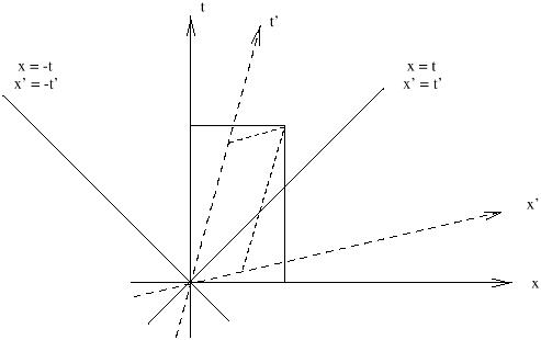
An extremely useful tool is the spacetime diagram, so let's
consider Minkowski space from this point of view. We can begin by
portraying the initial t and x axes at (what are
conventionally
thought of as) right angles, and suppressing the y and z axes.
Then according to (1.19), under a boost in the x-t plane
the x' axis (t' = 0) is given by
t = xtanh![]() , while the t' axis (x' = 0) is given by
t = x/tanh
, while the t' axis (x' = 0) is given by
t = x/tanh![]() . We therefore see that the space and time axes
are rotated into each other, although they scissor
together instead of remaining orthogonal in the traditional Euclidean
sense. (As we shall see, the axes do in fact remain orthogonal
in the Lorentzian sense.)
This should come as no surprise, since if spacetime behaved
just like a four-dimensional version of space the world would be a
very different place.
. We therefore see that the space and time axes
are rotated into each other, although they scissor
together instead of remaining orthogonal in the traditional Euclidean
sense. (As we shall see, the axes do in fact remain orthogonal
in the Lorentzian sense.)
This should come as no surprise, since if spacetime behaved
just like a four-dimensional version of space the world would be a
very different place.
|
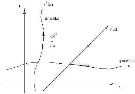
It is also enlightening to consider the paths corresponding to travel at the speed c = 1. These are given in the original coordinate system by x = ±t. In the new system, a moment's thought reveals that the paths defined by x' = ±t' are precisely the same as those defined by x = ±t; these trajectories are left invariant under Lorentz transformations. Of course we know that light travels at this speed; we have therefore found that the speed of light is the same in any inertial frame. A set of points which are all connected to a single event by straight lines moving at the speed of light is called a light cone; this entire set is invariant under Lorentz transformations. Light cones are naturally divided into future and past; the set of all points inside the future and past light cones of a point p are called timelike separated from p, while those outside the light cones are spacelike separated and those on the cones are lightlike or null separated from p. Referring back to (1.3), we see that the interval between timelike separated points is negative, between spacelike separated points is positive, and between null separated points is zero. (The interval is defined to be s2, not the square root of this quantity.) Notice the distinction between this situation and that in the Newtonian world; here, it is impossible to say (in a coordinate-independent way) whether a point that is spacelike separated from p is in the future of p, the past of p, or "at the same time".
To probe the structure of Minkowski space in more detail, it is necessary to introduce the concepts of vectors and tensors. We will start with vectors, which should be familiar. Of course, in spacetime vectors are four-dimensional, and are often referred to as four-vectors. This turns out to make quite a bit of difference; for example, there is no such thing as a cross product between two four-vectors.
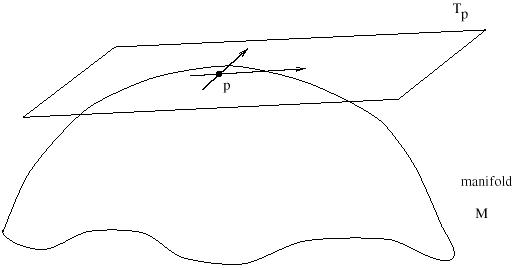
Beyond the simple fact of dimensionality, the most important thing to emphasize is that each vector is located at a given point in spacetime. You may be used to thinking of vectors as stretching from one point to another in space, and even of "free" vectors which you can slide carelessly from point to point. These are not useful concepts in relativity. Rather, to each point p in spacetime we associate the set of all possible vectors located at that point; this set is known as the tangent space at p, or Tp. The name is inspired by thinking of the set of vectors attached to a point on a simple curved two-dimensional space as comprising a plane which is tangent to the point. But inspiration aside, it is important to think of these vectors as being located at a single point, rather than stretching from one point to another. (Although this won't stop us from drawing them as arrows on spacetime diagrams.)
|
Later we will relate the tangent space at each point to things we can construct from the spacetime itself. For right now, just think of Tp as an abstract vector space for each point in spacetime. A (real) vector space is a collection of objects ("vectors") which, roughly speaking, can be added together and multiplied by real numbers in a linear way. Thus, for any two vectors V and W and real numbers a and b, we have

| (1.22) |
Every vector space has an origin, i.e. a zero vector which functions as an identity element under vector addition. In many vector spaces there are additional operations such as taking an inner (dot) product, but this is extra structure over and above the elementary concept of a vector space.
A vector is a perfectly well-defined geometric object, as is a vector field, defined as a set of vectors with exactly one at each point in spacetime. (The set of all the tangent spaces of a manifold M is called the tangent bundle, T(M).) Nevertheless it is often useful for concrete purposes to decompose vectors into components with respect to some set of basis vectors. A basis is any set of vectors which both spans the vector space (any vector is a linear combination of basis vectors) and is linearly independent (no vector in the basis is a linear combination of other basis vectors). For any given vector space, there will be an infinite number of legitimate bases, but each basis will consist of the same number of vectors, known as the dimension of the space. (For a tangent space associated with a point in Minkowski space, the dimension is of course four.)
Let us imagine that at each tangent space we set up a basis of four
vectors
![]() , with
, with
![]()
![]() {0, 1, 2, 3} as usual. In fact let us
say that each basis is adapted to the coordinates x
{0, 1, 2, 3} as usual. In fact let us
say that each basis is adapted to the coordinates x![]() ; that is, the
basis vector
; that is, the
basis vector
![]() is what we would normally think of pointing along
the x-axis, etc. It is by no means necessary that we choose a basis
which is adapted to any coordinate system at all, although it is often
convenient. (We really could be more precise here, but later
on we will repeat the discussion at an excruciating level of precision,
so some sloppiness now is forgivable.) Then any abstract vector
A can be written as a linear combination of basis vectors:
is what we would normally think of pointing along
the x-axis, etc. It is by no means necessary that we choose a basis
which is adapted to any coordinate system at all, although it is often
convenient. (We really could be more precise here, but later
on we will repeat the discussion at an excruciating level of precision,
so some sloppiness now is forgivable.) Then any abstract vector
A can be written as a linear combination of basis vectors:

| (1.23) |
The coefficients A![]() are the components of the vector
A.
More often than not we will forget the basis entirely and refer somewhat
loosely to "the vector A
are the components of the vector
A.
More often than not we will forget the basis entirely and refer somewhat
loosely to "the vector A![]() ", but keep in mind that this is
shorthand. The real vector is an abstract geometrical entity, while the
components are just the coefficients of the basis vectors in some
convenient basis. (Since we will usually suppress the explicit basis
vectors, the indices will usually label components of vectors and
tensors. This is why there are parentheses around the indices on the
basis vectors, to remind us that this is a collection of vectors, not
components of a single vector.)
", but keep in mind that this is
shorthand. The real vector is an abstract geometrical entity, while the
components are just the coefficients of the basis vectors in some
convenient basis. (Since we will usually suppress the explicit basis
vectors, the indices will usually label components of vectors and
tensors. This is why there are parentheses around the indices on the
basis vectors, to remind us that this is a collection of vectors, not
components of a single vector.)
A standard example of a vector in spacetime is the tangent vector to
a curve. A parameterized curve or path through spacetime is specified by
the coordinates as a function of the parameter, e.g.
x![]() (
(![]() ).
The tangent vector
V(
).
The tangent vector
V(![]() ) has components
) has components

| (1.24) |
The entire vector is thus
V = V![]()
![]() . Under a Lorentz transformation
the coordinates x
. Under a Lorentz transformation
the coordinates x![]() change according to (1.11), while the
parameterization
change according to (1.11), while the
parameterization ![]() is unaltered; we can therefore deduce that
the components of the tangent vector must change as
is unaltered; we can therefore deduce that
the components of the tangent vector must change as
| (1.25) |
However, the vector itself (as opposed to its components in some
coordinate system) is invariant under Lorentz transformations. We can
use this fact to derive the transformation properties of the basis
vectors. Let us refer to the set of basis vectors in the transformed
coordinate system as
![]() .
Since the vector is invariant, we have
.
Since the vector is invariant, we have
| (1.26) |
But this relation must hold no matter what the numerical values of
the components V![]() are. Therefore we can say
are. Therefore we can say
| (1.27) |
To get the new basis
![]() in terms of the old one
in terms of the old one
![]() we
should multiply by the inverse of the Lorentz transformation
we
should multiply by the inverse of the Lorentz transformation
![]()
![]() . But the inverse of a Lorentz
transformation
from the unprimed to the primed coordinates is also a Lorentz
transformation, this time from the primed to the unprimed systems.
We will therefore introduce a somewhat subtle notation, by writing
using the same symbol for both matrices, just with primed and unprimed
indices adjusted. That is,
. But the inverse of a Lorentz
transformation
from the unprimed to the primed coordinates is also a Lorentz
transformation, this time from the primed to the unprimed systems.
We will therefore introduce a somewhat subtle notation, by writing
using the same symbol for both matrices, just with primed and unprimed
indices adjusted. That is,
| (1.28) |
or
| (1.29) |
where
![]() is the traditional Kronecker delta symbol
in four dimensions. (Note that Schutz uses a different convention,
always arranging the two indices northwest/southeast; the important
thing is where the primes go.)
From (1.27) we then obtain the transformation rule for basis vectors:
is the traditional Kronecker delta symbol
in four dimensions. (Note that Schutz uses a different convention,
always arranging the two indices northwest/southeast; the important
thing is where the primes go.)
From (1.27) we then obtain the transformation rule for basis vectors:
| (1.30) |
Therefore the set of basis vectors transforms via the inverse Lorentz transformation of the coordinates or vector components.
It is worth pausing a moment to take all this in. We introduced
coordinates labeled by upper indices, which transformed in a certain
way under Lorentz transformations. We then considered vector components
which also were written with upper indices, which made sense since they
transformed in the same way as the coordinate functions. (In a fixed
coordinate system, each of the four coordinates x![]() can be thought
of as a function on spacetime, as can each of the four components of
a vector field.) The basis vectors associated with the coordinate
system transformed via the inverse matrix, and were labeled by a
lower index. This notation ensured that the invariant object constructed
by summing over the components and basis vectors was left unchanged by
the transformation, just as we would wish. It's probably not giving too
much away to say that this will continue to be the case for more
complicated objects with multiple indices (tensors).
can be thought
of as a function on spacetime, as can each of the four components of
a vector field.) The basis vectors associated with the coordinate
system transformed via the inverse matrix, and were labeled by a
lower index. This notation ensured that the invariant object constructed
by summing over the components and basis vectors was left unchanged by
the transformation, just as we would wish. It's probably not giving too
much away to say that this will continue to be the case for more
complicated objects with multiple indices (tensors).
Once we have set up a vector space, there is an associated vector space
(of equal dimension) which
we can immediately define, known as the dual vector space.
The dual space is usually denoted by an asterisk, so that the dual
space to the tangent space Tp is called the
cotangent space
and denoted T*p. The dual space is
the space of all linear maps from the original vector space to the real
numbers; in math lingo, if
![]()
![]() Tp* is a dual vector, then
it acts as a map such that:
Tp* is a dual vector, then
it acts as a map such that:

| (1.31) |
where V, W are vectors and a, b are real
numbers. The nice
thing about these maps is that they form a vector space themselves; thus,
if ![]() and
and ![]() are dual vectors, we have
are dual vectors, we have

| (1.32) |
To make this construction somewhat more concrete, we can introduce a
set of basis dual vectors
![]() by demanding
by demanding
| (1.33) |
Then every dual vector can be written in terms of its components, which we label with lower indices:

| (1.34) |
In perfect analogy with vectors, we will usually simply write
![]() to stand for the entire dual vector. In fact,
you will
sometime see elements of Tp (what we have called
vectors) referred
to as contravariant vectors, and elements of
Tp* (what we
have called dual vectors) referred to as covariant vectors. Actually,
if you just refer to ordinary vectors as vectors with upper indices
and dual vectors as vectors with lower indices, nobody should be
offended. Another name for dual vectors is one-forms, a somewhat
mysterious designation which will become clearer soon.
to stand for the entire dual vector. In fact,
you will
sometime see elements of Tp (what we have called
vectors) referred
to as contravariant vectors, and elements of
Tp* (what we
have called dual vectors) referred to as covariant vectors. Actually,
if you just refer to ordinary vectors as vectors with upper indices
and dual vectors as vectors with lower indices, nobody should be
offended. Another name for dual vectors is one-forms, a somewhat
mysterious designation which will become clearer soon.
The component notation leads to a simple way of writing the action of a dual vector on a vector:
| (1.35) |
This is why it is rarely necessary to write the basis vectors (and dual vectors) explicitly; the components do all of the work. The form of (1.35) also suggests that we can think of vectors as linear maps on dual vectors, by defining
| (1.36) |
Therefore, the dual space to the dual vector space is the original vector space itself.
Of course in spacetime we will be interested not in a single vector space, but in fields of vectors and dual vectors. (The set of all cotangent spaces over M is the cotangent bundle, T*(M).) In that case the action of a dual vector field on a vector field is not a single number, but a scalar (or just "function") on spacetime. A scalar is a quantity without indices, which is unchanged under Lorentz transformations.
We can use the same arguments that we earlier used for vectors to derive the transformation properties of dual vectors. The answers are, for the components,
| (1.37) |
and for basis dual vectors,
| (1.38) |
This is just what we would expect from index placement; the components of a dual vector transform under the inverse transformation of those of a vector. Note that this ensures that the scalar (1.35) is invariant under Lorentz transformations, just as it should be.
Let's consider some examples of dual vectors, first in other contexts and then in Minkowski space. Imagine the space of n-component column vectors, for some integer n. Then the dual space is that of n-component row vectors, and the action is ordinary matrix multiplication:
| (1.39) |
Another familiar example occurs in quantum mechanics, where vectors
in the Hilbert space are represented by kets,
|![]()
![]() . In this
case the dual space is the space of bras,
. In this
case the dual space is the space of bras,
![]()
![]() |, and the
action gives the number
|, and the
action gives the number
![]()
![]() |
|![]()
![]() . (This is a
complex number in quantum mechanics, but the idea is precisely the
same.)
. (This is a
complex number in quantum mechanics, but the idea is precisely the
same.)
In spacetime the simplest example of a dual vector is the gradient of a scalar function, the set of partial derivatives with respect to the spacetime coordinates, which we denote by "d":
| (1.40) |
The conventional chain rule used to transform partial derivatives amounts in this case to the transformation rule of components of dual vectors:
| (1.41) |
where we have used (1.11) and (1.28) to relate the Lorentz transformation to the coordinates. The fact that the gradient is a dual vector leads to the following shorthand notations for partial derivatives:
| (1.42) |
(Very roughly speaking, "x![]() has an upper index, but when it is in
the denominator of a derivative it implies a lower index on the resulting
object.") I'm not a big fan of the comma notation, but we will use
has an upper index, but when it is in
the denominator of a derivative it implies a lower index on the resulting
object.") I'm not a big fan of the comma notation, but we will use
![]() all the time. Note that the gradient does in fact act in a natural way
on the example we gave above of a vector, the tangent vector to a curve.
The result is ordinary derivative of the function along the curve:
all the time. Note that the gradient does in fact act in a natural way
on the example we gave above of a vector, the tangent vector to a curve.
The result is ordinary derivative of the function along the curve:
| (1.43) |
As a final note on dual vectors, there is a way to represent them as pictures which is consistent with the picture of vectors as arrows. See the discussion in Schutz, or in MTW (where it is taken to dizzying extremes).
A straightforward generalization of vectors and dual vectors is the notion of a tensor. Just as a dual vector is a linear map from vectors to R, a tensor T of type (or rank) (k, l ) is a multilinear map from a collection of dual vectors and vectors to R:
| (1.44) |
Here, "×" denotes the Cartesian product, so that for example Tp × Tp is the space of ordered pairs of vectors. Multilinearity means that the tensor acts linearly in each of its arguments; for instance, for a tensor of type (1, 1), we have

| (1.45) |
From this point of view, a scalar is a type (0, 0) tensor, a vector is a type (1, 0) tensor, and a dual vector is a type (0, 1) tensor.
The space of all tensors of a fixed type (k, l ) forms a
vector space;
they can be added together and multiplied by real numbers. To construct
a basis for this space, we need to define a new operation known as the
tensor product, denoted by ![]() . If T is a (k, l ) tensor
and S is a (m, n) tensor, we define a (k +
m, l + n) tensor
T
. If T is a (k, l ) tensor
and S is a (m, n) tensor, we define a (k +
m, l + n) tensor
T ![]() S by
S by

| (1.46) |
(Note that the
![]() and V(i) are distinct
dual vectors and vectors, not components thereof.)
In other words, first act T on the appropriate set of dual
vectors and
vectors, and then act S on the remainder, and then multiply the
answers. Note that, in general,
T
and V(i) are distinct
dual vectors and vectors, not components thereof.)
In other words, first act T on the appropriate set of dual
vectors and
vectors, and then act S on the remainder, and then multiply the
answers. Note that, in general,
T ![]() S
S ![]() S
S ![]() T.
T.
It is now straightforward to construct a basis for the space of all (k, l ) tensors, by taking tensor products of basis vectors and dual vectors; this basis will consist of all tensors of the form

| (1.47) |
In a 4-dimensional spacetime there will be 4k + l basis tensors in all. In component notation we then write our arbitrary tensor as

| (1.48) |
Alternatively, we could define the components by acting the tensor on basis vectors and dual vectors:

| (1.49) |
You can check for yourself, using (1.33) and so forth, that these equations all hang together properly.
As with vectors, we will usually take the shortcut of denoting the
tensor T by its components
T![]() ...
... ![]()
![]() ...
... ![]() .
The action of the tensors on a set of vectors and dual vectors follows
the pattern established in (1.35):
.
The action of the tensors on a set of vectors and dual vectors follows
the pattern established in (1.35):

| (1.50) |
The order of the indices is obviously important, since the tensor need not act in the same way on its various arguments. Finally, the transformation of tensor components under Lorentz transformations can be derived by applying what we already know about the transformation of basis vectors and dual vectors. The answer is just what you would expect from index placement,

| (1.51) |
Thus, each upper index gets transformed like a vector, and each lower index gets transformed like a dual vector.
Although we have defined tensors as linear maps from sets of vectors and tangent vectors to R, there is nothing that forces us to act on a full collection of arguments. Thus, a (1, 1) tensor also acts as a map from vectors to vectors:
| (1.52) |
You can check for yourself that
T![]()
![]() V
V![]() is a vector
( i.e. obeys the vector transformation law). Similarly, we
can act one tensor on (all or part of) another tensor to obtain
a third tensor. For example,
is a vector
( i.e. obeys the vector transformation law). Similarly, we
can act one tensor on (all or part of) another tensor to obtain
a third tensor. For example,
| (1.53) |
is a perfectly good (1, 1) tensor.
You may be concerned that this introduction to tensors has been somewhat
too brief, given the esoteric nature of the material. In fact, the
notion of tensors does not require a great deal of effort to master;
it's just a matter of keeping the indices straight, and the rules for
manipulating them are very natural. Indeed, a number of books like to
define tensors as collections of numbers transforming according to
(1.51). While this is operationally useful, it tends to obscure the
deeper meaning of tensors as geometrical entities with a life independent
of any chosen coordinate system. There is, however, one subtlety which
we have glossed over. The notions of dual vectors and tensors and bases
and linear maps belong to the realm of linear algebra, and are
appropriate whenever we have an abstract vector space at hand. In the
case of interest to us we have not just a vector space, but a vector
space at each point in spacetime. More often than not we are interested
in tensor fields, which can be thought of as tensor-valued functions on
spacetime. Fortunately, none of the manipulations we defined above
really care whether we are dealing with a single vector space or a
collection of vector spaces, one for each event. We will be able to
get away with simply calling things functions of x![]() when
appropriate. However, you should keep straight the logical independence
of the notions we have introduced and their specific application to
spacetime and relativity.
when
appropriate. However, you should keep straight the logical independence
of the notions we have introduced and their specific application to
spacetime and relativity.
Now let's turn to some examples of tensors. First we consider the
previous example of column vectors and their duals, row vectors. In
this system a (1, 1) tensor is simply a matrix,
Mij. Its action on a pair
(![]() , V) is given by usual matrix multiplication:
, V) is given by usual matrix multiplication:
| (1.54) |
If you like, feel free to think of tensors as "matrices with an arbitrary number of indices."
In spacetime, we have already seen some examples of tensors without
calling them that. The most familiar example of a (0, 2) tensor is
the metric,
![]() . The action of the metric on two vectors is
so useful that it gets its own name, the inner product (or
dot product):
. The action of the metric on two vectors is
so useful that it gets its own name, the inner product (or
dot product):
| (1.55) |
Just as with the conventional Euclidean dot product, we will refer to two vectors whose dot product vanishes as orthogonal. Since the dot product is a scalar, it is left invariant under Lorentz transformations; therefore the basis vectors of any Cartesian inertial frame, which are chosen to be orthogonal by definition, are still orthogonal after a Lorentz transformation (despite the "scissoring together" we noticed earlier). The norm of a vector is defined to be inner product of the vector with itself; unlike in Euclidean space, this number is not positive definite:
|
(A vector can have zero norm without being the zero vector.) You will notice that the terminology is the same as that which we earlier used to classify the relationship between two points in spacetime; it's no accident, of course, and we will go into more detail later.
Another tensor is the Kronecker delta
![]() , of type (1, 1),
which you already know the components of. Related to this and
the metric is the inverse metric
, of type (1, 1),
which you already know the components of. Related to this and
the metric is the inverse metric
![]() , a type (2, 0)
tensor defined as the inverse of the metric:
, a type (2, 0)
tensor defined as the inverse of the metric:
| (1.56) |
In fact, as you can check, the inverse metric has exactly the same components as the metric itself. (This is only true in flat space in Cartesian coordinates, and will fail to hold in more general situations.) There is also the Levi-Civita tensor, a (0, 4) tensor:
| (1.57) |
Here, a "permutation of 0123" is an ordering of the numbers 0, 1,
2, 3 which can be obtained by starting with 0123 and exchanging two of the
digits; an even permutation is obtained by an even number of such exchanges,
and an odd permutation is obtained by an odd number. Thus, for example,
![]() = - 1.
= - 1.
It is a remarkable property of the above tensors - the metric, the inverse metric, the Kronecker delta, and the Levi-Civita tensor - that, even though they all transform according to the tensor transformation law (1.51), their components remain unchanged in any Cartesian coordinate system in flat spacetime. In some sense this makes them bad examples of tensors, since most tensors do not have this property. In fact, even these tensors do not have this property once we go to more general coordinate systems, with the single exception of the Kronecker delta. This tensor has exactly the same components in any coordinate system in any spacetime. This makes sense from the definition of a tensor as a linear map; the Kronecker tensor can be thought of as the identity map from vectors to vectors (or from dual vectors to dual vectors), which clearly must have the same components regardless of coordinate system. The other tensors (the metric, its inverse, and the Levi-Civita tensor) characterize the structure of spacetime, and all depend on the metric. We shall therefore have to treat them more carefully when we drop our assumption of flat spacetime.
A more typical example of a tensor is the electromagnetic field
strength tensor. We all know that the electromagnetic fields are made up
of the electric field vector Ei and the magnetic field
vector Bi.
(Remember that we use Latin indices for spacelike components 1,2,3.)
Actually these are only "vectors" under rotations in space, not under
the full Lorentz group. In fact they are components of a (0, 2)
tensor
F![]()
![]() , defined by
, defined by
| (1.58) |
From this point of view it is easy to transform the electromagnetic fields in one reference frame to those in another, by application of (1.51). The unifying power of the tensor formalism is evident: rather than a collection of two vectors whose relationship and transformation properties are rather mysterious, we have a single tensor field to describe all of electromagnetism. (On the other hand, don't get carried away; sometimes it's more convenient to work in a single coordinate system using the electric and magnetic field vectors.)
With some examples in hand we can now be a little more systematic about some properties of tensors. First consider the operation of contraction, which turns a (k, l ) tensor into a (k - 1, l - 1) tensor. Contraction proceeds by summing over one upper and one lower index:
| (1.59) |
You can check that the result is a well-defined tensor. Of course it is only permissible to contract an upper index with a lower index (as opposed to two indices of the same type). Note also that the order of the indices matters, so that you can get different tensors by contracting in different ways; thus,
| (1.60) |
in general.
The metric and inverse metric can be used to raise and lower
indices on tensors. That is, given a tensor
T![]()
![]()
![]()
![]() , we can use the metric to define new
tensors which we choose to denote by the same letter T:
, we can use the metric to define new
tensors which we choose to denote by the same letter T:
| (1.61) |
and so forth. Notice that raising and lowering does not change the position of an index relative to other indices, and also that "free" indices (which are not summed over) must be the same on both sides of an equation, while "dummy" indices (which are summed over) only appear on one side. As an example, we can turn vectors and dual vectors into each other by raising and lowering indices:
| (1.62) |
This explains why the gradient in three-dimensional flat Euclidean space is usually thought of as an ordinary vector, even though we have seen that it arises as a dual vector; in Euclidean space (where the metric is diagonal with all entries +1) a dual vector is turned into a vector with precisely the same components when we raise its index. You may then wonder why we have belabored the distinction at all. One simple reason, of course, is that in a Lorentzian spacetime the components are not equal:
| (1.63) |
In a curved spacetime, where the form of the metric is generally more complicated, the difference is rather more dramatic. But there is a deeper reason, namely that tensors generally have a "natural" definition which is independent of the metric. Even though we will always have a metric available, it is helpful to be aware of the logical status of each mathematical object we introduce. The gradient, and its action on vectors, is perfectly well defined regardless of any metric, whereas the "gradient with upper indices" is not. (As an example, we will eventually want to take variations of functionals with respect to the metric, and will therefore have to know exactly how the functional depends on the metric, something that is easily obscured by the index notation.)
Continuing our compilation of tensor jargon, we refer to a tensor as symmetric in any of its indices if it is unchanged under exchange of those indices. Thus, if

| (1.64) |
we say that
S![]()
![]()
![]() is symmetric in its first two indices,
while if
is symmetric in its first two indices,
while if

| (1.65) |
we say that
S![]()
![]()
![]() is symmetric in all three of its indices.
Similarly, a tensor is antisymmetric (or "skew-symmetric") in
any of its indices if it changes sign when those indices are exchanged;
thus,
is symmetric in all three of its indices.
Similarly, a tensor is antisymmetric (or "skew-symmetric") in
any of its indices if it changes sign when those indices are exchanged;
thus,
| (1.66) |
means that
A![]()
![]()
![]() is antisymmetric in its first and third
indices (or just "antisymmetric in
is antisymmetric in its first and third
indices (or just "antisymmetric in ![]() and
and ![]() "). If a tensor
is (anti-) symmetric in all of its indices, we refer to it as simply
(anti-) symmetric (sometimes with the redundant modifier "completely").
As examples, the metric
"). If a tensor
is (anti-) symmetric in all of its indices, we refer to it as simply
(anti-) symmetric (sometimes with the redundant modifier "completely").
As examples, the metric
![]() and the inverse
metric
and the inverse
metric
![]() are symmetric, while the Levi-Civita tensor
are symmetric, while the Levi-Civita tensor
![]() and the electromagnetic field
strength tensor
F
and the electromagnetic field
strength tensor
F![]()
![]() are antisymmetric. (Check for yourself
that if you
raise or lower a set of indices which are symmetric or antisymmetric,
they remain that way.) Notice that it makes no sense to exchange upper
and lower indices with each other, so don't succumb to the temptation
to think of the Kronecker delta
are antisymmetric. (Check for yourself
that if you
raise or lower a set of indices which are symmetric or antisymmetric,
they remain that way.) Notice that it makes no sense to exchange upper
and lower indices with each other, so don't succumb to the temptation
to think of the Kronecker delta
![]() as symmetric.
On the other hand, the fact that lowering an index on
as symmetric.
On the other hand, the fact that lowering an index on
![]() gives a symmetric tensor (in fact, the metric) means that the order of
indices doesn't really matter, which is why we don't keep track index
placement for this one tensor.
gives a symmetric tensor (in fact, the metric) means that the order of
indices doesn't really matter, which is why we don't keep track index
placement for this one tensor.
Given any tensor, we can symmetrize (or antisymmetrize) any number of its upper or lower indices. To symmetrize, we take the sum of all permutations of the relevant indices and divide by the number of terms:

| (1.67) |
while antisymmetrization comes from the alternating sum:

| (1.68) |
By "alternating sum" we mean that permutations which are the result of an odd number of exchanges are given a minus sign, thus:

| (1.69) |
Notice that round/square brackets denote symmetrization/antisymmetrization. Furthermore, we may sometimes want to (anti-) symmetrize indices which are not next to each other, in which case we use vertical bars to denote indices not included in the sum:
| (1.70) |
Finally, some people use a convention in which the factor of 1/n! is omitted. The one used here is a good one, since (for example) a symmetric tensor satisfies
| (1.71) |
and likewise for antisymmetric tensors.
We have been very careful so far to distinguish clearly between things that are always true (on a manifold with arbitrary metric) and things which are only true in Minkowski space in Cartesian coordinates. One of the most important distinctions arises with partial derivatives. If we are working in flat spacetime with Cartesian coordinates, then the partial derivative of a (k, l ) tensor is a (k, l + 1) tensor; that is,
| (1.72) |
transforms properly under Lorentz transformations. However, this will
no longer be true in more general spacetimes, and we will have to
define a "covariant derivative" to take the place of the partial
derivative. Nevertheless, we can still use the fact that partial
derivatives give us tensor in this special case, as long as we keep
our wits about us. (The one exception to this warning is the partial
derivative of a scalar,
![]()
![]() , which is a perfectly
good tensor [the gradient] in any spacetime.)
, which is a perfectly
good tensor [the gradient] in any spacetime.)
We have now accumulated enough tensor know-how to illustrate some of these concepts using actual physics. Specifically, we will examine Maxwell's equations of electrodynamics. In 19th-century notation, these are
| (1.73) |
Here, E and B are the electric and magnetic field
3-vectors, J is the current, ![]() is the charge density, and
is the charge density, and
![]() × and
× and
![]() . are the conventional curl and divergence.
These equations are invariant under Lorentz transformations, of course;
that's how the whole business got started. But they don't look obviously
invariant; our tensor notation can fix that. Let's begin by writing
these equations in just a slightly different notation,
. are the conventional curl and divergence.
These equations are invariant under Lorentz transformations, of course;
that's how the whole business got started. But they don't look obviously
invariant; our tensor notation can fix that. Let's begin by writing
these equations in just a slightly different notation,
| (1.74) |
In these expressions, spatial indices have been raised and lowered
with abandon, without any attempt to keep straight where the metric
appears. This is because
![]() is the metric on flat 3-space,
with
is the metric on flat 3-space,
with ![]() its inverse (they are equal as matrices). We can
therefore raise and lower indices at will, since the components don't
change. Meanwhile,
the three-dimensional Levi-Civita tensor
its inverse (they are equal as matrices). We can
therefore raise and lower indices at will, since the components don't
change. Meanwhile,
the three-dimensional Levi-Civita tensor
![]() is defined
just as the four-dimensional one, although with one fewer index. We
have replaced the charge density by J0; this is
legitimate because
the density and current together form the current 4-vector,
J
is defined
just as the four-dimensional one, although with one fewer index. We
have replaced the charge density by J0; this is
legitimate because
the density and current together form the current 4-vector,
J![]() = (
= (![]() , J1, J2,
J3).
, J1, J2,
J3).
From these expressions, and the definition (1.58) of the field strength
tensor
F![]()
![]() , it is easy to get a completely tensorial
20th-century version of Maxwell's equations. Begin by noting
that we can express the field strength with upper indices as
, it is easy to get a completely tensorial
20th-century version of Maxwell's equations. Begin by noting
that we can express the field strength with upper indices as
| (1.75) |
(To check this, note for example that
F01 = ![]()
![]() F01 and
F12 =
F01 and
F12 = ![]() B3.) Then the first two
equations in (1.74) become
B3.) Then the first two
equations in (1.74) become
| (1.76) |
Using the antisymmetry of
F![]()
![]() , we see that these may be combined
into the single tensor equation
, we see that these may be combined
into the single tensor equation
| (1.77) |
A similar line of reasoning, which is left as an exercise to you, reveals that the third and fourth equations in (1.74) can be written

| (1.78) |
The four traditional Maxwell equations are thus replaced by two, thus demonstrating the economy of tensor notation. More importantly, however, both sides of equations (1.77) and (1.78) manifestly transform as tensors; therefore, if they are true in one inertial frame, they must be true in any Lorentz-transformed frame. This is why tensors are so useful in relativity - we often want to express relationships without recourse to any reference frame, and it is necessary that the quantities on each side of an equation transform in the same way under change of coordinates. As a matter of jargon, we will sometimes refer to quantities which are written in terms of tensors as covariant (which has nothing to do with "covariant" as opposed to "contravariant"). Thus, we say that (1.77) and (1.78) together serve as the covariant form of Maxwell's equations, while (1.73) or (1.74) are non-covariant.
Let us now introduce a special class of tensors, known as
differential forms (or just "forms"). A differential
p-form is a (0, p) tensor which is completely antisymmetric.
Thus, scalars are automatically 0-forms, and dual vectors are automatically
one-forms (thus explaining this terminology from a while back). We also
have the 2-form
F![]()
![]() and the 4-form
and the 4-form
![]() .
The space of all p-forms is denoted
.
The space of all p-forms is denoted ![]() , and the space of all
p-form fields over a manifold M is denoted
, and the space of all
p-form fields over a manifold M is denoted
![]() (M).
A semi-straightforward exercise in combinatorics reveals that the number
of linearly independent p-forms on an n-dimensional vector
space is
n!/(p!(n - p)!). So at a point on a
4-dimensional spacetime there is one linearly independent 0-form,
four 1-forms, six 2-forms, four 3-forms, and one 4-form. There
are no p-forms for p > n, since all of the
components will automatically be zero by antisymmetry.
(M).
A semi-straightforward exercise in combinatorics reveals that the number
of linearly independent p-forms on an n-dimensional vector
space is
n!/(p!(n - p)!). So at a point on a
4-dimensional spacetime there is one linearly independent 0-form,
four 1-forms, six 2-forms, four 3-forms, and one 4-form. There
are no p-forms for p > n, since all of the
components will automatically be zero by antisymmetry.
Why should we care about differential forms? This is a hard question to answer without some more work, but the basic idea is that forms can be both differentiated and integrated, without the help of any additional geometric structure. We will delay integration theory until later, but see how to differentiate forms shortly.
Given a p-form A and a q-form B, we can form
a (p + q)-form
known as the wedge product A ![]() B by taking the antisymmetrized
tensor product:
B by taking the antisymmetrized
tensor product:
| (1.79) |
Thus, for example, the wedge product of two 1-forms is

| (1.80) |
Note that
| (1.81) |
so you can alter the order of a wedge product if you are careful with signs.
The exterior derivative "d" allows us to differentiate p-form fields to obtain (p + 1)-form fields. It is defined as an appropriately normalized antisymmetric partial derivative:

| (1.82) |
The simplest example is the gradient, which is the exterior derivative of a 1-form:

| (1.83) |
The reason why the exterior derivative deserves special attention is that it is a tensor, even in curved spacetimes, unlike its cousin the partial derivative. Since we haven't studied curved spaces yet, we cannot prove this, but (1.82) defines an honest tensor no matter what the metric and coordinates are.
Another interesting fact about exterior differentiation is that, for any form A,

| (1.84) |
which is often written
d2 = 0. This identity is a consequence of
the definition of d and the fact that partial derivatives commute,
![]()
![]() =
= ![]()
![]() (acting on anything). This leads
us to the following mathematical aside, just for fun.
We define a p-form A to be closed if
dA = 0, and exact if
A = dB for some (p - 1)-form B. Obviously,
all exact forms are
closed, but the converse is not necessarily true. On a manifold M,
closed p-forms comprise a vector space
Zp(M), and exact forms
comprise a vector space Bp(M). Define a new
vector space as the closed forms modulo the exact forms:
(acting on anything). This leads
us to the following mathematical aside, just for fun.
We define a p-form A to be closed if
dA = 0, and exact if
A = dB for some (p - 1)-form B. Obviously,
all exact forms are
closed, but the converse is not necessarily true. On a manifold M,
closed p-forms comprise a vector space
Zp(M), and exact forms
comprise a vector space Bp(M). Define a new
vector space as the closed forms modulo the exact forms:
| (1.85) |
This is known as the pth de Rham cohomology vector space,
and depends
only on the topology of the manifold M. (Minkowski space is
topologically
equivalent to R4, which is uninteresting, so that all
of the
Hp(M) vanish for p > 0; for p
= 0 we have H0(M) = ![]() .
Therefore in Minkowski space all closed forms
are exact except for zero-forms; zero-forms can't be exact since
there are no -1-forms for them to be the exterior derivative of.)
It is striking that information about the topology can be extracted in
this way, which essentially involves the solutions to differential
equations. The dimension bp of the space
Hp(M) is called the pth
Betti number of M, and the Euler characteristic is given by the
alternating sum
.
Therefore in Minkowski space all closed forms
are exact except for zero-forms; zero-forms can't be exact since
there are no -1-forms for them to be the exterior derivative of.)
It is striking that information about the topology can be extracted in
this way, which essentially involves the solutions to differential
equations. The dimension bp of the space
Hp(M) is called the pth
Betti number of M, and the Euler characteristic is given by the
alternating sum
| (1.86) |
Cohomology theory is the basis for much of modern differential topology.
Moving back to reality, the final operation on differential forms we will introduce is Hodge duality. We define the "Hodge star operator" on an n-dimensional manifold as a map from p-forms to (n - p)-forms,
| (1.87) |
mapping A to "A dual". Unlike our other operations on forms, the Hodge dual does depend on the metric of the manifold (which should be obvious, since we had to raise some indices on the Levi-Civita tensor in order to define (1.87)). Applying the Hodge star twice returns either plus or minus the original form:
| (1.88) |
where s is the number of minus signs in the eigenvalues of the metric (for Minkowski space, s = 1).
Two facts on the Hodge dual: First, "duality" in the sense of Hodge is different than the relationship between vectors and dual vectors, although both can be thought of as the space of linear maps from the original space to R. Notice that the dimensionality of the space of (n - p)-forms is equal to that of the space of p-forms, so this has at least a chance of being true. In the case of forms, the linear map defined by an (n - p)-form acting on a p-form is given by the dual of the wedge product of the two forms. Thus, if A(n - p) is an (n - p)-form and B(p) is a p-form at some point in spacetime, we have
| (1.89) |
The second fact concerns differential forms in 3-dimensional Euclidean space. The Hodge dual of the wedge product of two 1-forms gives another 1-form:
| (1.90) |
(All of the prefactors cancel.) Since 1-forms in Euclidean space are just like vectors, we have a map from two vectors to a single vector. You should convince yourself that this is just the conventional cross product, and that the appearance of the Levi-Civita tensor explains why the cross product changes sign under parity (interchange of two coordinates, or equivalently basis vectors). This is why the cross product only exists in three dimensions - because only in three dimensions do we have an interesting map from two dual vectors to a third dual vector. If you wanted to you could define a map from n - 1 one-forms to a single one-form, but I'm not sure it would be of any use.
Electrodynamics provides an especially compelling example of the use
of differential forms. From the definition of the exterior derivative,
it is clear that equation (1.78) can be concisely expressed as closure
of the two-form
F![]()
![]() :
:

| (1.91) |
Does this mean that F is also exact? Yes; as we've noted, Minkowski
space is topologically trivial, so all closed forms are exact. There
must therefore be a one-form A![]() such that
such that

| (1.92) |
This one-form is the familiar vector potential of electromagnetism,
with the 0 component given by the scalar potential,
A0 = ![]() .
If one starts from the view that the A
.
If one starts from the view that the A![]() is the fundamental field
of electromagnetism, then (1.91) follows as an identity (as opposed to a
dynamical law, an equation of motion). Gauge invariance is expressed
by the observation that the theory is invariant under
A
is the fundamental field
of electromagnetism, then (1.91) follows as an identity (as opposed to a
dynamical law, an equation of motion). Gauge invariance is expressed
by the observation that the theory is invariant under
A ![]() A + d
A + d![]() for some scalar (zero-form)
for some scalar (zero-form) ![]() , and this is also
immediate from the relation (1.92). The
other one of Maxwell's equations, (1.77), can be expressed as an equation
between three-forms:
, and this is also
immediate from the relation (1.92). The
other one of Maxwell's equations, (1.77), can be expressed as an equation
between three-forms:
| (1.93) |
where the current one-form J is just the current four-vector with index lowered. Filling in the details is left for you to do.
As an intriguing aside, Hodge duality is the basis for one of the hottest
topics in theoretical physics today. It's hard not to notice that the
equations (1.91) and (1.93) look very similar. Indeed, if we set
J![]() = 0,
the equations are invariant under the "duality transformations"
= 0,
the equations are invariant under the "duality transformations"

| (1.94) |
We therefore say that the vacuum Maxwell's equations are duality
invariant, while the invariance is spoiled in the presence of charges.
We might imagine that magnetic as well as electric monopoles existed in
nature; then we could add a magnetic current term
4![]() (*JM) to the
right hand side of (1.91), and the equations would be invariant under
duality transformations plus the additional replacement
J
(*JM) to the
right hand side of (1.91), and the equations would be invariant under
duality transformations plus the additional replacement
J ![]() JM.
(Of course a nonzero right hand side to (1.91) is inconsistent with
F = dA,
so this idea only works if A
JM.
(Of course a nonzero right hand side to (1.91) is inconsistent with
F = dA,
so this idea only works if A![]() is not a fundamental variable.)
Long ago Dirac considered the idea of magnetic monopoles and showed that
a necessary condition for their existence is that the fundamental
monopole charge be inversely proportional to the fundamental electric
charge. Now, the fundamental electric charge is a small number;
electrodynamics is "weakly coupled", which is why perturbation theory
is so remarkably successful in quantum electrodynamics (QED). But
Dirac's condition on magnetic charges implies that a duality
transformation takes a theory of weakly coupled electric charges to
a theory of strongly coupled magnetic monopoles (and vice-versa).
Unfortunately monopoles don't exist (as far as we know), so these
ideas aren't directly applicable to electromagnetism; but there are
some theories (such as supersymmetric non-abelian gauge theories) for
which it has been long conjectured that some sort of duality symmetry
may exist. If it did, we would have the opportunity to analyze a
theory which looked strongly coupled (and therefore hard to solve) by
looking at the weakly coupled dual version. Recently work by Seiberg
and Witten and others has provided very strong evidence that this is
exactly what happens in certain theories. The hope is that these
techniques will allow us to explore various phenomena which we know
exist in strongly coupled quantum field theories, such as confinement
of quarks in hadrons.
is not a fundamental variable.)
Long ago Dirac considered the idea of magnetic monopoles and showed that
a necessary condition for their existence is that the fundamental
monopole charge be inversely proportional to the fundamental electric
charge. Now, the fundamental electric charge is a small number;
electrodynamics is "weakly coupled", which is why perturbation theory
is so remarkably successful in quantum electrodynamics (QED). But
Dirac's condition on magnetic charges implies that a duality
transformation takes a theory of weakly coupled electric charges to
a theory of strongly coupled magnetic monopoles (and vice-versa).
Unfortunately monopoles don't exist (as far as we know), so these
ideas aren't directly applicable to electromagnetism; but there are
some theories (such as supersymmetric non-abelian gauge theories) for
which it has been long conjectured that some sort of duality symmetry
may exist. If it did, we would have the opportunity to analyze a
theory which looked strongly coupled (and therefore hard to solve) by
looking at the weakly coupled dual version. Recently work by Seiberg
and Witten and others has provided very strong evidence that this is
exactly what happens in certain theories. The hope is that these
techniques will allow us to explore various phenomena which we know
exist in strongly coupled quantum field theories, such as confinement
of quarks in hadrons.
We've now gone over essentially everything there is to know about the care and feeding of tensors. In the next section we will look more carefully at the rigorous definitions of manifolds and tensors, but the basic mechanics have been pretty well covered. Before jumping to more abstract mathematics, let's review how physics works in Minkowski spacetime.
Start with the worldline of a single particle. This is specified
by a map
![]()
![]() M, where M is the manifold representing
spacetime; we usually think of the path as a parameterized curve
x
M, where M is the manifold representing
spacetime; we usually think of the path as a parameterized curve
x![]() (
(![]() ). As mentioned earlier, the tangent vector to this
path is
dx
). As mentioned earlier, the tangent vector to this
path is
dx![]() /d
/d![]() (note that it depends on the parameterization).
An object of primary interest is the norm
of the tangent vector, which serves to characterize the path; if the
tangent vector is timelike/null/spacelike at some parameter value
(note that it depends on the parameterization).
An object of primary interest is the norm
of the tangent vector, which serves to characterize the path; if the
tangent vector is timelike/null/spacelike at some parameter value
![]() , we say that the path is timelike/null/spacelike at that
point. This explains why the same words are used to classify vectors
in the tangent space and intervals between two points - because a
straight line connecting, say, two timelike separated points will
itself be timelike at every point along the path.
, we say that the path is timelike/null/spacelike at that
point. This explains why the same words are used to classify vectors
in the tangent space and intervals between two points - because a
straight line connecting, say, two timelike separated points will
itself be timelike at every point along the path.
|
Nevertheless, it's important to be aware of the sleight of hand which is being pulled here. The metric, as a (0, 2) tensor, is a machine which acts on two vectors (or two copies of the same vector) to produce a number. It is therefore very natural to classify tangent vectors according to the sign of their norm. But the interval between two points isn't something quite so natural; it depends on a specific choice of path (a "straight line") which connects the points, and this choice in turn depends on the fact that spacetime is flat (which allows a unique choice of straight line between the points). A more natural object is the line element, or infinitesimal interval:
| (1.95) |
From this definition it is tempting to take the square root and integrate along a path to obtain a finite interval. But since ds2 need not be positive, we define different procedures for different cases. For spacelike paths we define the path length
| (1.96) |
where the integral is taken over the path. For null paths the interval is zero, so no extra formula is required. For timelike paths we define the proper time
| (1.97) |
which will be positive. Of course we may consider paths that are
timelike in some places and spacelike in others, but fortunately
it is seldom necessary since the paths of physical particles never
change their character (massive particles move on timelike paths,
massless particles move on null paths). Furthermore, the phrase
"proper time" is especially appropriate, since ![]() actually
measures the time elapsed on a physical clock carried along the path.
This point of view makes the "twin paradox" and similar puzzles
very clear; two worldlines, not necessarily straight, which intersect at
two different events in spacetime will have proper times measured by the
integral (1.97) along the appropriate paths, and these two numbers will
in general be different even if the people travelling along them were
born at the same time.
actually
measures the time elapsed on a physical clock carried along the path.
This point of view makes the "twin paradox" and similar puzzles
very clear; two worldlines, not necessarily straight, which intersect at
two different events in spacetime will have proper times measured by the
integral (1.97) along the appropriate paths, and these two numbers will
in general be different even if the people travelling along them were
born at the same time.
Let's move from the consideration of paths in general to the paths
of massive particles (which will always be timelike). Since the proper
time is measured by a clock travelling on a timelike worldline,
it is convenient to use ![]() as the parameter along the path.
That is, we use (1.97) to compute
as the parameter along the path.
That is, we use (1.97) to compute
![]() (
(![]() ), which (if
), which (if ![]() is a good parameter in the first place) we can invert to obtain
is a good parameter in the first place) we can invert to obtain
![]() (
(![]() ), after which we can think of the path as
x
), after which we can think of the path as
x![]() (
(![]() ). The tangent vector in this parameterization is known
as the four-velocity, U
). The tangent vector in this parameterization is known
as the four-velocity, U![]() :
:

| (1.98) |
Since d![]() = -
= - ![]() dx
dx![]() dx
dx![]() , the four-velocity is
automatically normalized:
, the four-velocity is
automatically normalized:
| (1.99) |
(It will always be negative, since we are only defining it for timelike
trajectories. You could define an analogous vector for spacelike
paths as well; null paths give some extra problems since the norm is
zero.) In the rest frame of a particle, its four-velocity has
components
U![]() = (1, 0, 0, 0).
= (1, 0, 0, 0).
A related vector is the energy-momentum four-vector, defined by

| (1.100) |
where m is the mass of the particle. The mass is a fixed quantity
independent of inertial frame; what you may be used to thinking of as
the "rest mass." It turns out to be much more convenient to take
this as the mass once and for all, rather than thinking of mass as
depending on velocity. The energy of a particle is simply
p0, the timelike component of its energy-momentum vector.
Since it's only one component of a four-vector, it is not invariant
under Lorentz transformations; that's to be expected, however, since
the energy of a particle at rest is not the same as that of the same
particle in motion. In the
particle's rest frame we have p0 = m; recalling
that we have set
c = 1, we find that we have found the equation that made Einstein
a celebrity, E = mc2. (The field equations of
general relativity are
actually much more important than this one, but "
R![]()
![]() -
- ![]() Rg
Rg![]()
![]() = 8
= 8![]() GT
GT![]()
![]() " doesn't elicit the visceral reaction that
you get from "E = mc2".) In a moving frame we
can find the components
of p
" doesn't elicit the visceral reaction that
you get from "E = mc2".) In a moving frame we
can find the components
of p![]() by performing a Lorentz transformation;
for a particle
moving with (three-) velocity v along the x axis we have
by performing a Lorentz transformation;
for a particle
moving with (three-) velocity v along the x axis we have
| (1.101) |
where
![]() = 1/
= 1/![]() . For small v, this gives
p0 = m +
. For small v, this gives
p0 = m + ![]() mv2 (what we usually think of as
rest energy
plus kinetic energy) and p1 = mv (what we
usually think of as
[Newtonian] momentum). So the energy-momentum vector lives up to its name.
mv2 (what we usually think of as
rest energy
plus kinetic energy) and p1 = mv (what we
usually think of as
[Newtonian] momentum). So the energy-momentum vector lives up to its name.
The centerpiece of pre-relativity physics is Newton's 2nd Law, or
![]() = m
= m![]() = d
= d![]() /dt. An analogous equation should hold
in SR, and the requirement that it be tensorial leads us directly
to introduce a force four-vector f
/dt. An analogous equation should hold
in SR, and the requirement that it be tensorial leads us directly
to introduce a force four-vector f![]() satisfying
satisfying
| (1.102) |
The simplest example of a force in Newtonian physics is the force
due to gravity. In relativity, however, gravity is not described
by a force, but rather by the curvature of spacetime itself. Instead,
let us consider electromagnetism. The three-dimensional Lorentz
force is given by
![]() = q(
= q(![]() +
+ ![]() ×
× ![]() ),
where q is the charge on the particle. We would like a tensorial
generalization of this equation. There turns out to be a unique answer:
),
where q is the charge on the particle. We would like a tensorial
generalization of this equation. There turns out to be a unique answer:
| (1.103) |
You can check for yourself that this reduces to the Newtonian version in the limit of small velocities. Notice how the requirement that the equation be tensorial, which is one way of guaranteeing Lorentz invariance, severely restricted the possible expressions we could get. This is an example of a very general phenomenon, in which a small number of an apparently endless variety of possible physical laws are picked out by the demands of symmetry.
Although p![]() provides a complete description of the
energy and
momentum of a particle, for extended systems it is necessary to go
further and define the energy-momentum tensor (sometimes called
the stress-energy tensor),
T
provides a complete description of the
energy and
momentum of a particle, for extended systems it is necessary to go
further and define the energy-momentum tensor (sometimes called
the stress-energy tensor),
T![]()
![]() . This is a symmetric (2, 0) tensor
which tells us all we need to know about the energy-like aspects of a
system: energy density, pressure, stress, and so
forth. A general definition of
T
. This is a symmetric (2, 0) tensor
which tells us all we need to know about the energy-like aspects of a
system: energy density, pressure, stress, and so
forth. A general definition of
T![]()
![]() is "the flux of four-momentum
p
is "the flux of four-momentum
p![]() across a surface of constant
x
across a surface of constant
x![]() ". To make this more
concrete, let's consider the very general category of matter which
may be characterized as a fluid - a continuum of matter
described by macroscopic quantities such as temperature, pressure,
entropy, viscosity, etc. In fact this definition is so general that
it is of little use. In general relativity essentially all interesting
types of matter can be thought of as perfect fluids, from
stars to electromagnetic fields to the entire universe. Schutz
defines a perfect fluid to be one with no heat conduction and no
viscosity, while Weinberg defines it as a fluid which looks isotropic
in its rest frame; these two viewpoints turn out to be equivalent.
Operationally, you should think of a perfect fluid as one which may
be completely characterized by its pressure and density.
". To make this more
concrete, let's consider the very general category of matter which
may be characterized as a fluid - a continuum of matter
described by macroscopic quantities such as temperature, pressure,
entropy, viscosity, etc. In fact this definition is so general that
it is of little use. In general relativity essentially all interesting
types of matter can be thought of as perfect fluids, from
stars to electromagnetic fields to the entire universe. Schutz
defines a perfect fluid to be one with no heat conduction and no
viscosity, while Weinberg defines it as a fluid which looks isotropic
in its rest frame; these two viewpoints turn out to be equivalent.
Operationally, you should think of a perfect fluid as one which may
be completely characterized by its pressure and density.
To understand perfect fluids, let's start with the even simpler example
of dust. Dust is defined as a collection of particles at rest
with respect to each other, or alternatively as a perfect fluid with
zero pressure. Since the particles all have an equal velocity in
any fixed inertial frame, we can imagine a "four-velocity field"
U![]() (x) defined all over
spacetime. (Indeed, its components are
the same at each point.) Define the number-flux four-vector
to be
(x) defined all over
spacetime. (Indeed, its components are
the same at each point.) Define the number-flux four-vector
to be

| (1.104) |
where n is the number density of the particles as measured in their rest frame. Then N0 is the number density of particles as measured in any other frame, while Ni is the flux of particles in the xi direction. Let's now imagine that each of the particles have the same mass m. Then in the rest frame the energy density of the dust is given by

| (1.105) |
By definition, the energy density completely specifies the dust. But
![]() only measures the energy density in the rest frame; what
about
other frames? We notice that both n and m are 0-components of
four-vectors in their rest frame; specifically,
N
only measures the energy density in the rest frame; what
about
other frames? We notice that both n and m are 0-components of
four-vectors in their rest frame; specifically,
N![]() = (n, 0, 0, 0) and
p
= (n, 0, 0, 0) and
p![]() = (m, 0, 0, 0). Therefore
= (m, 0, 0, 0). Therefore ![]() is the
is the ![]() = 0,
= 0,
![]() = 0 component of the tensor
p
= 0 component of the tensor
p ![]() N as measured in its
rest frame. We are therefore led to define the energy-momentum tensor
for dust:
N as measured in its
rest frame. We are therefore led to define the energy-momentum tensor
for dust:

| (1.106) |
where ![]() is defined as the energy density in the rest frame.
is defined as the energy density in the rest frame.
Having mastered dust, more general perfect fluids are not much more
complicated. Remember that "perfect" can be taken to mean
"isotropic in its rest frame." This in turn means that
T![]()
![]() is diagonal - there is no net flux of any component of momentum
in an orthogonal direction. Furthermore, the nonzero spacelike
components must all be equal,
T11 = T22 =
T33. The only
two independent numbers are therefore T00 and one of the
Tii; we can choose to call the first of these the
energy density
is diagonal - there is no net flux of any component of momentum
in an orthogonal direction. Furthermore, the nonzero spacelike
components must all be equal,
T11 = T22 =
T33. The only
two independent numbers are therefore T00 and one of the
Tii; we can choose to call the first of these the
energy density
![]() , and the second the pressure p. (Sorry that it's
the same
letter as the momentum.) The energy-momentum tensor of a perfect
fluid therefore takes the following form in its rest frame:
, and the second the pressure p. (Sorry that it's
the same
letter as the momentum.) The energy-momentum tensor of a perfect
fluid therefore takes the following form in its rest frame:
| (1.107) |
We would like, of course, a formula which is good in any frame.
For dust we had
T![]()
![]() =
= ![]() U
U![]() U
U![]() , so we might begin by
guessing
(
, so we might begin by
guessing
(![]() + p)U
+ p)U![]() U
U![]() , which gives
, which gives
| (1.108) |
To get the answer we want we must therefore add
| (1.109) |
Fortunately, this has an obvious covariant generalization, namely
p![]() . Thus, the general form of the energy-momentum
tensor for a perfect fluid is
. Thus, the general form of the energy-momentum
tensor for a perfect fluid is
| (1.110) |
This is an important formula for applications such as stellar structure and cosmology.
As further examples, let's consider the energy-momentum tensors of electromagnetism and scalar field theory. Without any explanation at all, these are given by
| (1.111) |
and

| (1.112) |
You can check for yourself that, for example, T00 in each case is equal to what you would expect the energy density to be.
Besides being symmetric,
T![]()
![]() has the even more important property
of being conserved. In this context, conservation is
expressed as the vanishing of the "divergence":
has the even more important property
of being conserved. In this context, conservation is
expressed as the vanishing of the "divergence":

| (1.113) |
This is a set of four equations, one for each value of ![]() . The
. The
![]() = 0 equation corresponds to conservation of energy, while
= 0 equation corresponds to conservation of energy, while
![]() T
T![]() k = 0 expresses conservation of the
kth
component of the momentum. We are not going to prove this in
general; the proof follows for any individual source of matter from
the equations of motion obeyed by that kind of matter. In fact, one
way to define
T
k = 0 expresses conservation of the
kth
component of the momentum. We are not going to prove this in
general; the proof follows for any individual source of matter from
the equations of motion obeyed by that kind of matter. In fact, one
way to define
T![]()
![]() would be "a (2, 0) tensor with units of
energy per volume, which is conserved." You can prove conservation
of the energy-momentum tensor for electromagnetism, for example, by
taking the divergence of (1.111) and using Maxwell's equations
as previously discussed.
would be "a (2, 0) tensor with units of
energy per volume, which is conserved." You can prove conservation
of the energy-momentum tensor for electromagnetism, for example, by
taking the divergence of (1.111) and using Maxwell's equations
as previously discussed.
A final aside: we have already mentioned that in general relativity gravitation does not count as a "force." As a related point, the gravitational field also does not have an energy-momentum tensor. In fact it is very hard to come up with a sensible local expression for the energy of a gravitational field; a number of suggestions have been made, but they all have their drawbacks. Although there is no "correct" answer, it is an important issue from the point of view of asking seemingly reasonable questions such as "What is the energy emitted per second from a binary pulsar as the result of gravitational radiation?"