


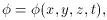
It is completely in the spirit of general field theory to assume that a
quantity  that is defined
everywhere and at every instant of time exists.
This rather vague statement, which can be written in the usual
coordinates as
that is defined
everywhere and at every instant of time exists.
This rather vague statement, which can be written in the usual
coordinates as
does not exclude the case
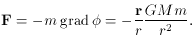
where G is the Newtonian gravitational constant G = 0.57 x
10-8 cm3 g-1 s-2. The
derivative of the potential determines the force
which acts on a body with mass m:
As is well known, when we generalize the Newtonian theory to
distributions of mass it takes the form of the Poisson equation
where
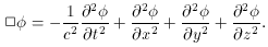
We now apply special relativity. The Newton and Poisson
formulations imply that the field
In mathematics, it is well known that the solutions of<
By setting
Therefore, the right-hand side of the equation (i.e., f) must also be
a scalar. This means that the source of the scalar field, the "scalar field
charge", is also a scalar. Furthermore, it cannot be a particle volume
density!
The second point, which we already used in writing the generalized
equation, is that we could put the scalar
In order to come to an understanding of how scalar field theory
works, we shall discuss two simple exact solutions. The first is
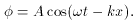
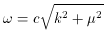
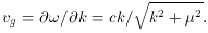
It may easily be seen that for
and arbitrary amplitude A, (5.7) is a solution to the free-field
(f = 0)
equation. This is a completely new property that the Newtonian scalar
gravitational field does not possess. The new relativistic equation for
This does not violate relativity theory: the group velocity
vg, i.e., the
velocity at which an impulse is propagated, determines the speed of
information propagation. As is well known,
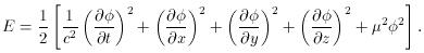
The energy density of the classical scalar field is given by the following
expression:
The energy density is always positive and behaves like the
T44
component of the energy-momentum tensor; this formula like the other
versions of the theory (some special
V(
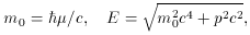
By virtue of the equivalence formula E = mc2, we can
say that the particles have a mass
so that the term µ introduced in (5.7) is the quantum
mechanical rest
mass of the particles corresponding to the solution of (5.7) (up to a
trivial factor of
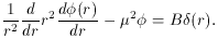
We now turn to the second simple solution. Assume a static
time-independent point source at the origin, f = B
The solution to (5.14) is
So the second effect resulting from the insertion of µ in
the right-hand
side of the basic equation is that the interaction has a cutoff at a
distance r0 = µ-1; by comparison with
the Newton and Coulomb laws,
But once again we must emphasize that the most important qualitative
difference (which is due to the fact that the vector electromagnetic
potential has a time component) between the electrostatic field and a
true scalar field is present even in the case µ = 0. The difference
is that
equal charges repel one another in the electrostatic case, while equal
charges attract one another in the scalar case. A related effect is that a
point electric charge has infinite positive energy, while a point scalar
charge has infinite negative energy (in the classical theory).
The fact that equal charges attract one another in scalar field theory
makes it similar to Newtonian gravitation, but, as mentioned above,
detailed study shows that real gravitation (as in celestial mechanics) is
not a scalar field.
We shall return to the mechanical picture of the scalar field below
(Section 7), after a short historical note
(Section 6).
5 n is the volume density of
electrons; e is their charge. In the general case of different
particles,
 = 0 in
some regions of space-time or
-> 0 asymptotically as the spatial
coordinates do go to infinity. As
mentioned above, the Newtonian theory of gravitation uses precisely
such a quantity: the gravitational potential outside a mass M,
= 0 in
some regions of space-time or
-> 0 asymptotically as the spatial
coordinates do go to infinity. As
mentioned above, the Newtonian theory of gravitation uses precisely
such a quantity: the gravitational potential outside a mass M,


 is the mass density in
g cm-3. For a star, this
equation results
in a smooth function (without an
infinity in the center of the star)
inside the star and solution (5.2) outside the star. We now assume that
perhaps other potentials, with somewhat different properties (see
immediately below), whose strength depends on a new type of special
"scalar" charge density q instead of
, exist. We assume the existence
of an independent scalar field (or fields) of nongravitational origin.
at each point in space depends on the
position of the mass (or the mass distribution) at the same instant of
time. The left- and right-hand sides of the Poisson equations are
assumed to be evaluated at the same instant of time. This flagrantly
contradicts the fundamental idea that the speed c (the speed of light,
3 x 1010 cm s-1) is the limiting speed for all
transfers of energy,
momentum, or information. In order to make the Poisson equation
comply with relativity, we must replace the
is the mass density in
g cm-3. For a star, this
equation results
in a smooth function (without an
infinity in the center of the star)
inside the star and solution (5.2) outside the star. We now assume that
perhaps other potentials, with somewhat different properties (see
immediately below), whose strength depends on a new type of special
"scalar" charge density q instead of
, exist. We assume the existence
of an independent scalar field (or fields) of nongravitational origin.
at each point in space depends on the
position of the mass (or the mass distribution) at the same instant of
time. The left- and right-hand sides of the Poisson equations are
assumed to be evaluated at the same instant of time. This flagrantly
contradicts the fundamental idea that the speed c (the speed of light,
3 x 1010 cm s-1) is the limiting speed for all
transfers of energy,
momentum, or information. In order to make the Poisson equation
comply with relativity, we must replace the
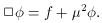
 2 (Laplacian)
with a
2 (Laplacian)
with a  (d'Alembertian):
 = f with
= 0 at t =
-
= f with
= 0 at t =
- propagate from the source
toward the future at the speed of light.
=
(x, y, z, t), we tacitly
assume that it is a four-scalar:
in a given place x, y, z at a given instant of time t, it
is the same for every
observer; it does not change if the observer is moving, i.e., under a
Lorentz transformation. This is not as trivial as it seems at first glance.
If there is a distribution of electric charge
=
ne, (5) we
must ask if the
charge is at rest or, in other words, if there is an electric current present
as well. Even if there is no current in one frame of reference, a moving
observer will observe a current and the values of the charge density
will be transformed: ' =
/ sqrt[1 -
propagate from the source
toward the future at the speed of light.
=
(x, y, z, t), we tacitly
assume that it is a four-scalar:
in a given place x, y, z at a given instant of time t, it
is the same for every
observer; it does not change if the observer is moving, i.e., under a
Lorentz transformation. This is not as trivial as it seems at first glance.
If there is a distribution of electric charge
=
ne, (5) we
must ask if the
charge is at rest or, in other words, if there is an electric current present
as well. Even if there is no current in one frame of reference, a moving
observer will observe a current and the values of the charge density
will be transformed: ' =
/ sqrt[1 -
 2]. In
fact, is the
time component
of a four-vector and is not a scalar. In contrast, this is not the case for
the function . We explicitly assume
that is not transformed, so that
is a scalar - a four-scalar in
Minkowski space. In general, the
derivatives of are not scalars. In
particular,
ð / ðt is
the time component and grad is the
space component of a four-vector. None of
these derivatives are invariant; none of the second derivatives are either,
with one important exception. The d'Alembertian
is a scalar! It is
a scalar in four-dimensional space in the same way that the Laplacian
2
is a scalar in three-dimensional space.
itself (multiplied by some
constant denoted by µ2) in the right-hand side. Even
more generally,
one could use V(), an
arbitrary scalar function V of the
scalar . In
this case, the scalar field is called a self-interacting scalar field. This
V-term is not used in the simplest case, with
µ2 , because
it leads to a linear equation:
2]. In
fact, is the
time component
of a four-vector and is not a scalar. In contrast, this is not the case for
the function . We explicitly assume
that is not transformed, so that
is a scalar - a four-scalar in
Minkowski space. In general, the
derivatives of are not scalars. In
particular,
ð / ðt is
the time component and grad is the
space component of a four-vector. None of
these derivatives are invariant; none of the second derivatives are either,
with one important exception. The d'Alembertian
is a scalar! It is
a scalar in four-dimensional space in the same way that the Laplacian
2
is a scalar in three-dimensional space.
itself (multiplied by some
constant denoted by µ2) in the right-hand side. Even
more generally,
one could use V(), an
arbitrary scalar function V of the
scalar . In
this case, the scalar field is called a self-interacting scalar field. This
V-term is not used in the simplest case, with
µ2 , because
it leads to a linear equation:
 allows the field to propagate like
a wave; this property did not exist
in the Newton-Poisson approximation. By standard well-known
methods, one can show that the phase velocity
allows the field to propagate like
a wave; this property did not exist
in the Newton-Poisson approximation. By standard well-known
methods, one can show that the phase velocity
 ) instead of
1/2 µ2
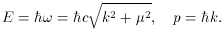
2) is basic; its
cosmological importance will be discussed below. By quantizing the
plane wave solution, one finds that the wave can be treated as a
collection of particles ("quanta"), where each particle has the following
characteristics:
) instead of
1/2 µ2
2) is basic; its
cosmological importance will be discussed below. By quantizing the
plane wave solution, one finds that the wave can be treated as a
collection of particles ("quanta"), where each particle has the following
characteristics:
 /c). The
waves are longitudinal; the y
and z
components of grad are not
involved in the propagation along the x-axis
- compare this with a similar electromagnetic wave, which would be
transverse: Ey = Hz =
/c). The
waves are longitudinal; the y
and z
components of grad are not
involved in the propagation along the x-axis
- compare this with a similar electromagnetic wave, which would be
transverse: Ey = Hz =
 A cos
( t -
kx). The scalar field has no
intrinsic angular momentum, and the particles are called scalar
particles.
A cos
( t -
kx). The scalar field has no
intrinsic angular momentum, and the particles are called scalar
particles.
 /r. It is easy to find a
static (time-independent), spherically symmetric solution for
.
Equation (5.6) reduces to
/r. It is easy to find a
static (time-independent), spherically symmetric solution for
.
Equation (5.6) reduces to


=
 niei. Back.