C. Inflation and Scalar Fields

As stated above, inflation is capable of solving many of the initial value, or `fine-tuning', problems of the hot Big Bang model. This is assuming that there is some mechanism to bring about the negative pressure state needed for quasi-exponential growth of the scale factor. In the early 1980's, Alan Guth [33] was studying properties of grand unified theories or GUTs. He noticed that these theories predict a large number of topological defects. Specifically, he was addressing the issue of monopole creation in the SU(5) GUT. He found the theory predicts a large number of these monopoles, and that they should `over-close' the universe. This means that the monopole contribution to is greater than the observed upper-bound on the density parameter, > 4, which comes from observation [5]. To remedy this, Guth concluded that the symmetry breaking associated with scalar fields in the particle theory must cause the universe to enter a period of rapid expansion. This expansion `dilutes' the density of the monopoles created, as stated above.

The first step in understanding the dynamics of scalar fields is to undertake the study of field theory. In field theory, one considers a Lagrangian density, as opposed to the usual Lagrangian from classical mechanics. This is because the scalar field is taken to be a continuous field, whereas the Lagrangian in mechanics is usually based on discrete particle systems. The Lagrangian (L) is related to the Lagrangian density () by,

(52)

Usually the scalar field is represented by a continuous function, (x, t), which can be real or complex. Given a potential density of the field, V(), takes the form,

(53)

The resulting Euler-Lagrange equations result from varying the action with respect to spacetime [41],

(54)

where x^µ = (t, -xⁱ) as usual, and = c = 1. Also note, g_µ = diag(1, -1, -1, -1), the factor of -g that usually appears in the action and other equations involving tensor densities will be sqrt[-(-1)] = 1 (Minkowski space). The resulting equation is

(55)

The prime represents differentiation with respect to and the term containing the Hubble constant serves as a kind of friction term resulting from the expansion. The field is taken to be homogeneous, which eliminates any gradient contributions. This homogeneity is a safe assumption, since physical gradients are related to comoving gradients by the scale factor,

(56)

Thus, the inhomogeneities in the field are redshifted away during inflation since the scale factor increases by a large amount.

One can also define the stress-energy tensor by use of Noether's theorem [41],

(57)

This is useful, because it can be compared to T^µ for a perfect fluid, namely,

The calculation for the pressure is a bit more subtle,

Consider the first component of pressure, again making use of (53) and (57),

Since g¹¹ = -1 and one can use the metric to raise and lower indices,

Since the metric is diagonal this yields,

Similarly, the T²² and T³³ components may be found. So for the total pressure one finds,

or,

(58)

From the T⁰⁰ component we already found,

(59)

Equations (58), (59) for the pressure and the energy density, show that the equation, p = - is not quite satisfied. A first resolution to this problem is to again assume that the scalar field () is spatially homogeneous, allowing one to eliminate the gradient terms (). This assumption is only made at this point to simplify the analysis. As we have seen if one keeps the terms, it can be shown that the gradients are redshifted away by the expansion (56). Ignoring gradients, the equations become

(60)

(61)

The first term 1/2 ² can be thought of as the kinetic energy and the second as the potential, or configuration energy. It is now possible to explicitly see where Equation (55) came from if we assume the field can be described as a `perfect' fluid. This assumption allows us to use a continuity equation,

(62)

By plugging in the energy density of the field (61) and making use of the Friedmann equation (to get H) one obtains Equation (55) in perhaps a more enlightening way.

From the pressure and energy density derived above, we see that the requirement that p = - can be approximately met, if one requires << V(). This leads to what is called the slow-roll approximation (SRA), which provides a natural condition for inflation to occur ⁽²⁵⁾ To assure the constraint on , one must also require that be negligible. Given these requirements, we will to define the slow-roll parameters and introduce the Planck mass ⁽²⁶⁾ [46],

(63)

(64)

At this point, it is useful to distinguish as the inflaton field. Inflaton is the name given to , since its origin does not have to originate with a specified particle theory. Although the original hope was that would help determine the correct particle physics models, current model building does not necessarily require specific particle phenomenology. This is actually an advantage for inflation, it retains its power to solve the initial value problems, yet it could arise from any arbitrary source (i.e., any arbitrary inflaton).

However, observation of the large-scale structure of the universe and anisotropies in the cosmic background should be able to constrain the inflaton parameters to a particular region. This can then be used by particle theorists, as a motivation for some required scalar field. Observational aspects of inflation will be considered in the next section, but this property of the inflaton field manifests itself as one of the greatest contributions of cosmology commensurate with particle theory. Some examples of potentials that have been proposed for the inflaton are presented below [47], [29].

(65)

(66)

(67)

(68)

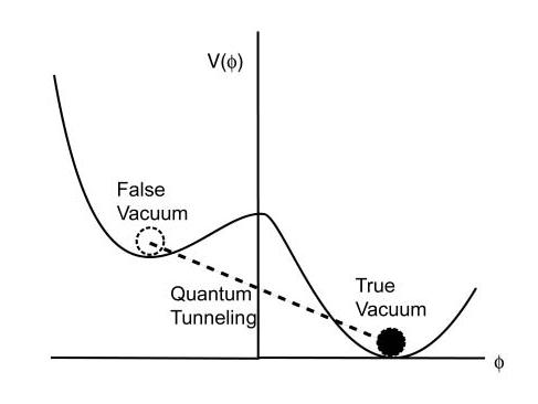
In Guth's original inflation scenario [33], the inflaton field () sits at a local minimum and is trapped in a false vacuum state (see Figure 7). The vacuum state of a field or particle is the lowest energy state available to the system. Some examples are the ground state of the hydrogen atom (-13.6 eV) and the ground state of the harmonic oscillator (1/2 ). The concept of `false' vacuum comes from examination of Figure 7. If is `placed' in the potential well on the left, the lowest energy available is that of the false vacuum. The only way can get out of this local minimum is by quantum tunneling, after some characteristic time. As tunneling takes place the universe inflates. Inflation halts when reaches the false vacuum and bubbles of the false vacuum coalesce releasing the `latent' heat that was stored in the field. This is much like the way bubble nucleation occurs when opening a bottle of compressed liquid (like soda). Energy escapes from the soda in the form of carbon dioxide and the liquid enters a lower more favorable energy state.

Figure 7. Toy Model For Original Inflaton. In this model of inflation the inflaton finds itself trapped in a false minimum. It is freed from this minimum when tunneling is allowed to occur resulting in a first order phase transition in the early universe.

Tunneling that leads to bubble nucleation is a first order phase transition. This is very similar to processes that take place in the study of condensed matter physics, fluid dynamics, and ferromagnetism (see for example [48] and [49]). The bubbles experience a state of negative pressure. Once created, they continue to expand at an exponential rate. Each expanding bubble corresponds to an expanding domain. However, when one carefully investigates this situation, one finds that the bubbles can collide as they reach the false vacuum. Furthermore, the size of these bubbles expands at too great of a rate and the corresponding universe is left void of structure. One finds that too much inflation occurs and the visible universe is left empty. This is referred to as the `graceful exit' problem. Again one is presented with an empty universe, which was the same reason that the DeSitter universe idea was abandoned.

Guth and others further tried to remedy these problems by fine-tuning the bubble formation. The problem with this is two fold. One, cosmologists and particle theorists don't like fine-tuning. The idea is to form a model that gives our universe as a usual result that follows from natural consequences. By natural one means that the scales of the model are related to the fundamental constants of nature; e.g., quantum gravity should occur at the Planck scale, since this scale is the only one natural in units (c, , G). Secondly, if the model is fine-tuned to agree with the observations of the anisotropies in the cosmic background, the bubbles would collide far too often. This results in the appearance of topological defects, like the monopoles. However, this was the whole reason inflation was invoked in the first place.

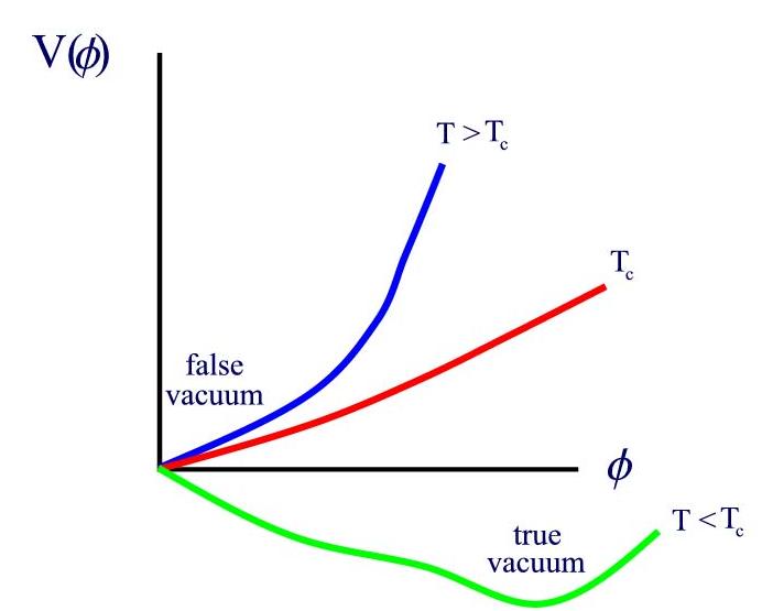
In 1982, a solution to the graceful exit problem was proposed by Linde [50] and independently by Steinhardt and Albrecht [51]. This New Inflation model solves the graceful exit problem by assuming the inflaton field evolves very slowly from its initial state, while undergoing a phase transition of second order. Figure 8 illustrates this by again considering the evolution of . If `rolls' down the potential at a slow rate, one obtains the amount of inflation needed to solve the initial value problems. After the universe cools to a critical temperature, T<sub>c</sub>, can proceed to its `true' vacuum state energy. The transition of the potential is a second order phase transition, so this model does not require tunneling [42]. This type of transition is similar to the transitions that occur in ferromagnetic systems [49].

Figure 8. Toy Model For New Inflation - When the temperature of the universe decreases to the critical temperature Tc, the scalar field potential experiences a second order phase transition. This makes the `true' vacuum state available to .

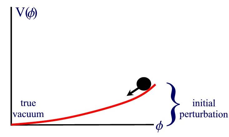
The majority of current models rely on another concept coined by Linde as Chaotic Inflation. This model differs from Old and New Inflation in that no phase transitions occur. In this scenario the inflaton is displaced from its true vacuum state by some arbitrary mechanism, perhaps quantum or thermal fluctuations. Given this initial state, the inflaton slowly rolls down the potential returning to the true vacuum (see Figure 9). This model has the advantage that no fine-tuning of critical temperature is required. This model presents a scenario, which can be fulfilled by a number of different models.

Figure 9. Toy Model For Chaotic Inflation - The inflaton finds itself displaced from the true vacuum and proceeds to `roll' back. Inflation takes place while the inflaton is displaced.

²⁵ In much of the literature on inflation, the slow-roll approximation is presented as a necessary and sufficient condition for inflation. However, in many new models of inflation this is not necessary. For a treatment of these models, see [43], [44], [45, and references therein]. Back.
²⁶ The Planck mass is easier to work with opposed to Newton's constant G, since most of the interesting energy scales are on the order of GeV (1 eV = 1.6 x 10^-19 Joules). In these units, the Planck mass is 10¹⁹ GeV. Back.