2.2 Correlation testing

Let us now consider the formal tests for correlation. To do so, we have to make the initial choice - parametric or non-parametric? The parametric tests are a little more powerful (a formal term - see Section 4.1), but not a lot; and they assume that the underlying probability distribution is known. On a fishing expedition. This matter may be well outside our control. The non-parametric tests are safest in such instances, permitting, in addition, tests on data which are not numerically defined (binned data, or ranked data), so that in some cases they may be the only alternative.

A parametric test for correlation. The standard parametric test assumes that the variables (x_i, y_i) are Normally distributed. The statistic computed is the Pearson product moment correlation coefficient (Fisher 1944):

where there are N data pairs x_i = x_i(obs) - (obs) and y_i = y_i(obs) -(obs), the barred quantities representing the means of the sample.

The standard deviation in r is

Note that -1 < r < 1; r = 0 for no correlation. To test the significance of a non-zero value for r, compute

which obeys the probability distribution of the ``Students'' t statistic ⁽¹⁾, with N - 2 degrees of freedom. We are hypothesis testing now, and the methodology is described more systematically in Section 4.1. Basically, we are testing the (null) hypothesis that the two variables are unrelated; rejection of this hypothesis will demonstrate that the variables are correlated.

Consult Table A I, the table of critical values for t; if t exceeds that corresponding to a critical value of the probability (two-tailed test), then the hypothesis that the variables are unrelated can be rejected at the specified level of significance. This level of significance (say 1 or 5 per cent) is the maximum probability we are willing to risk in deciding to reject the null hypothesis (no correlation) when it is in fact true.

Non-parametric tests for correlation. If the test is between data that are Normally distributed, or are known to be close to Normal distribution, then r is the appropriate correlation coefficient. If the distributions are unknown, however, as is frequently the case for astronomical statistics, then a non-parametric test must be used. The best known of these consists of computing the Spearman rank correlation coefficient (Conover 1980; Siegel & Castellan 1988):

where there are N data pairs, and the N values of each of the two variables are ranked so that the (x_i, y_i) pairs represent the ranks of the variables for the ith pair, 1 < x_i < N, 1 < y_i < N.

The range is 0 < r_S < 1; a high value indicates significant correlation. To find out how significant, refer the computed r_S to Table A II, a table of critical values of r_S applicable for 4 N 50. If r_S exceeds an appropriate critical value, the hypothesis that the variables are unrelated is rejected at that level of significance. If N exceeds 50, compute

a statistic whose distribution for large N asymptotically approaches that of the t statistic with N - 2 degrees of freedom. The significance of t_r may be found from Table A I, and this represents the associated probability under the hypothesis that the variables are unrelated.

How does the use of r_S compare with use of r, the most powerful parametric test for correlation? Very well: the efficiency is 91 per cent. This means that if we apply r_S to a population for which we have a data pair (x_i, y_i) for each object and both variables are Normally distributed, we will need on average 100 (x_i, y_i) pairs for r_S to reveal that correlation at the same level of significance that r attains for 91 (x_i, y_i) pairs. The moral of the story is that if in doubt, little is lost by going for the non-parametric test.

An example of ``correlation'' at the notorious 2 level is shown in Fig. 2. Here, r_S = 0.28, N = 55 and the hypothesis that the variables are unrelated is rejected at the 5 per cent level of significance.

Fig. 2. An application of the Spearman rank test. V / Vmax is plotted against high-frequency spectral index for a complete sample of QSOs from the Parkes 2.7-GHz survey (Masson & Wall 1977). The Spearman rank correlation coefficient indicates a correlation at the 5 per cent level of significance in the sense that the flat-spectrum (low HF) QSOs have stochastically lower V / Vmax - or a more uniform spatial distribution - than do the steep-spectrum QSOs.

The Kendall rank correlation coefficient does the same as r_S, and with the same efficiency (Siegel & Castellan 1988).

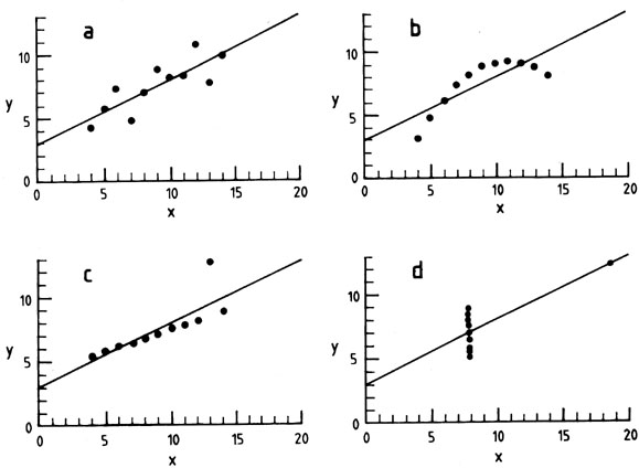
But what next? As a last warning in looking at relations between data pairs, I show Anscombe's (1973) quartet in Fig. 3. Here we have four fictitious sets of 11 (x_i, y_i). Each of the four has the same (, ), has identical coefficients of regression, and has the same regression line, residuals in y and estimated standard error in slope. Anscombe's point is the essential role of graphs in good statistical analysis. However, the examples illustrate other matters: the rule of thumb, and the distinction between independence of data points and correlation. In more than one of Anscombe's sets the data points are clearly related. They are far from independent, while not showing a particularly strong (formal) correlation.

Fig. 3. Anscombe's quartet. Each fictitious data set has II (x, y) pairs, the same mean * = 9 and mean * = 7.5, the same regression coefficient (y on x) of 0.5, the same equation of regression line y = 3 + 0.5x, sum of squares of x, and estimated standard error on regression coefficient.

If, however, we have demonstrated a correlation, it is logical to ask what the correlation is, i.e. what is the law that relates the variables. Quoting the answer is easy. Simply apply the so-called method of least squares to obtain the so-called regression line, y = ax + b, parameters a and b coming from the formula; see Section 3.1 below.

However, some things might worry us ⁽²⁾.

1. Why should least squares be correct? Are there better quantities to minimize? Will they give the same answer? And how ``parametric'' is this process?

2. What are the errors in a and b? The statement made in Paper I was that no quantity is of the slightest use unless it has an error of measurement associated; likewise for any quantity derived from the data. We must know the uncertainties.

3. Why should the line be linear? What is to stop us redesigning the axes and fitting exponentials or logarithmic curves by using linear regression? On the fishing expedition in which we have just discovered this ``deep and meaningful relationship'' - there is no limit in this respect; see Section 3.1 below. Fig. 3(b) is an example in which a linear fit is of indifferent quality, while choice of the ``correct'' relation would result in a perfect fit.

4. If we do not know what is the cause and effect with our correlation, which is the correct least-squares line: x on y or y on x? The coefficients are different. The lines are different. Which one is ``correct''? (There is an illustration of this conundrum in Burbidge 1979.) The answer is that it does not matter, as we are not testing physical hypotheses in this process. The regression lines are merely predictive, preferably with interpolation, and for example ``x on y'' would be chosen as the regression line if x is the variable to be predicted. (Indeed to avoid a judgemental approach of cause and effect, it is now common to consider orthogonal or bisector regression lines in order to incorporate uncertainties on both variables.)

The questions are getting bigger; and we have got into deep waters. Our simple hunt for correlation has led us into the game of model fitting, a game in which there are (fortunately) many powerful methods available to us but (unfortunately) many shades of opinion about how to proceed. The crucial point to bear in mind is: what did we set out to do? What was the original hypothesis?

This is the danger of the fishing trip. Perhaps we did not know what we were doing; we started with no hypothesis. It therefore should not surprise us that the significance of the result we find is difficult to assess. What is critical to keep clear is that examining data for correlation(s) is hypothesis testing, while estimating the relation is model fitting or data modelling, something entirely different.

² The first of these might be why this is called regression analysis. Galton (1889) introduced the term: it is from his examination of the inheritance of stature. He found that the sons of fathers who deviate x inches from the mean height of all fathers themselves deviate from the mean height of all sons by less than x inches. There is what Galton termed a ``regression to mediocrity''. The mathematicians who took up his challenge to analyse the correlation propagated his mediocre term and we are stuck with it. Back.