1.2. RESULTS

A simple analysis of cosmological perturbations can be obtained from a consideration of the Newtonian approximation to a homogeneous and isotropic universe. Consider a test particle at radius R from an arbitrary center. Because the model is homogeneous the choice of center does not matter. The evolution of the velocity of the test particle is given by the energy equation

(1.1)

If the total energy E_tot is positive, the Universe will expand forever since M, the mass (plus energy) enclosed within R, is positive, G is positive, and R is positive. In the absence of a cosmological constant or "dark energy," the expansion of the Universe will stop, leading to a recollapse if E_tot is negative. But this simple connection between E_tot and the fate of the Universe is broken in the presence of a vacuum energy density. The mass M is proportional to R³ because the Universe is homogeneous and the Hubble velocity is given by = HR. Thus E_tot R².

We can find the total energy by plugging in the velocity ₀ = H₀ R₀ and the density ₀ in the Universe now. This gives

(1.2)

with the critical density at time t₀ being _crit = 3 H₀² / (8 G). We define the ratio of density to critical density as = / _crit. This includes all forms of matter and energy. _m will be used to refer to the matter density.

From Equation 1.1 we can compute the time variation of . Let

(1.3)

If we divide this equation by 8 G R²/3 we get

(1.4)

Thus ^-1 - 1 ( R²)^-1. When declines with expansion at a rate faster than R^-2 then the deviation of from unity grows with expansion. This is the situation during the matter-dominated epoch with R^-3, so ^-1 - 1 R. During the radiation-dominated epoch R^-4, so ^-1 - 1 R². For ₀ to be within 0.9 and 1.1, needed to be between 0.999 and 1.001 at the epoch of recombination, and within 10^-15 of unity during nucleosynthesis. This fine-tuning problem is an aspect of the "flatness-oldness" problem in cosmology.

Inflation produces such a huge expansion that quantum fluctuations on the microscopic scale can grow to be larger than the observable Universe. These perturbations can be the seeds of structure formation and also will create the anisotropies seen by COBE for spherical harmonic indices 2. For perturbations that are larger than ~ c_s t (or ~ c_s / H) we can ignore pressure gradients, since pressure gradients produce sound waves that are not able to cross the perturbation in a Hubble time. In the absence of pressure gradients, the density perturbation will evolve in the same way that a homogeneous universe does, and we can use the equation

(1.5)

the assumption that 1 for early times, and << as indicated by the smallness of the T's seen by COBE, to derive

(1.6)

Hence,

(1.7)

where L is the comoving size of the perturbation. This is independent of the scale factor, so it does not change due to the expansion of the Universe.

During inflation (Guth 2003), the Universe is approximately in a steady state with constant H. Thus, the magnitude of for perturbations with physical scale c/H will be the same for all times during the inflationary epoch. But since this constant physical scale is aL, and the scale factor a changes by more than 30 orders of magnitude during inflation, this means that the magnitude of will be the same over 30 decades of comoving scale L. Thus, we get a strong prediction that will be the same on all observable scales from c / H₀ down to the scale that is no longer always larger than the sound speed horizon. This means that

(1.8)

so the Universe becomes extremely homogeneous on large scales even though it is quite inhomogeneous on small scales.

This behavior of being independent of scale is called equal power on all scales. It was originally predicted by Harrison (1970), Zel'dovich (1972), and Peebles & Yu (1970) based on a very simple argument: there is no scale length provided by the early Universe, and thus the perturbations should be scale-free - a power law. Therefore L^m. The gravitational potential divided by c² is a component of the metric, and if it gets comparable to unity then wild things happen. If m < 0 then gets large for small L, and many black holes would form. But we observe that this did not happen. Therefore m 0. But if m > 0 then gets large on large scales, and the Universe would be grossly inhomogeneous. But we observe that this is not the case, so m 0. Combining both results requires that m = 0, which is a scale-invariant perturbation power spectrum. This particular power-law power spectrum is called the Harrison-Zel'dovich spectrum. It was expected that the primordial perturbations should follow a Harrison-Zel'dovich spectrum because all other answers were wrong, but the inflationary scenario provides a good mechanism for producing a Harrison-Zel'dovich spectrum.

Sachs & Wolfe (1967) show that a gravitational potential perturbation produces an anisotropy of the CMB with magnitude

(1.9)

where is evaluated at the intersection of the line-of-sight and the surface of last scattering (or recombination at z 1100). The (1/3) factor arises because clocks run faster by a factor (1 + / c²) in a gravitational potential, and we can consider the expansion of the Universe to be a clock. Since the scale factor is varying as a t^2/3 at recombination, the faster expansion leads to a decreased temperature by T / T = -(2/3) / c², which, when added to the normal gravitational redshift T / T = / c² yields the (1/3) factor above. This is an illustration of the "gauge" problem in calculating perturbations in general relativity. The expected variation of the density contrast as the square of the scale factor for scales larger than the horizon in the radiation-dominated epoch is only obtained after allowance is made for the effect of the potential on the time. For a plane wave with wavenumber k we have -k² = 4 G , or

(1.10)

so when _crit at recombination, the Sachs-Wolfe effect exceeds the physical temperature fluctuation T / T = (1/4) / by a factor of 2(H / ck)² if fluctuations are adiabatic (all component number densities varying by the same factor).

In addition to the physical temperature fluctuation and the gravitational potential fluctuation, there is a Doppler shift term. When the baryon fluid has a density contrast given by

(1.11)

where c_s is the sound speed, then

(1.12)

As a result the velocity perturbation is given by = -c_sb. But the sound speed is given by c_s = (P / )^1/2 = [(4/3)c² / (3_b + 4)]^1/2 c / 3^1/2, since > _b at recombination (z = 1100). But the photon density is only slightly higher than the baryon density at recombination so the sound speed is about 20% smaller than c / 3^1/2. The Doppler shift term in the anisotropy is given by T / T = / c, as expected. This results in T / T slightly less than _b / 3^1/2, which is nearly 3^1/2 larger than the physical temperature fluctuation given by T / T = _b / 3.

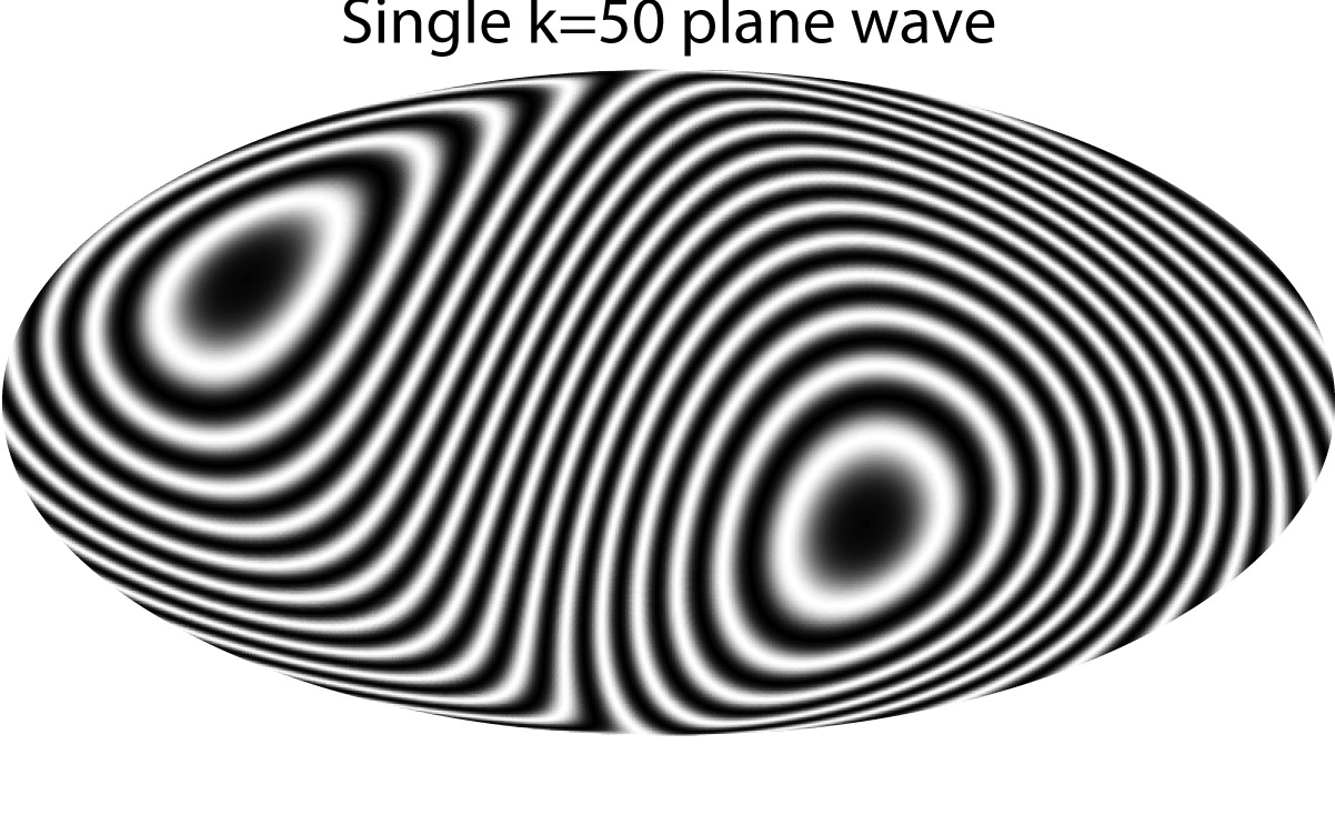
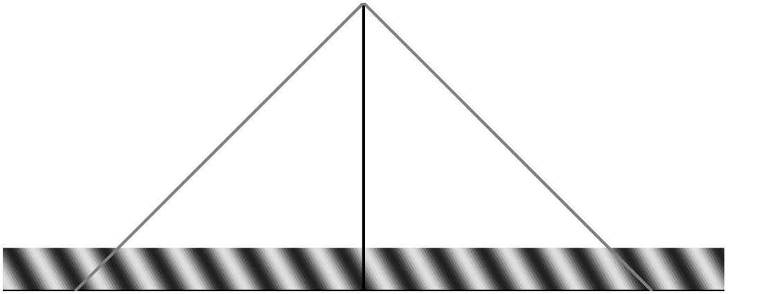
These plane-wave calculations need to be projected onto the sphere that is the intersection of our past light cone and the hypersurface corresponding to the time of recombination. Figure 1.2 shows a plane wave on these surfaces. The scalar density and potential perturbations produce a different pattern on the observed sky than the vector velocity perturbation. Figure 1.3 shows these patterns on the sky for a plane wave with k R_LS = 50, where R_LS is the radius of the last-scattering surface. The contribution of the velocity term is multiplied by cos, and since the RMS of this over the sphere is (1/3)^1/2, the RMS contribution of the velocity term almost equals the RMS contribution from the density term since the speed of sound is almost c/3^1/2.

Figure 1.2. A plane wave on the last-scattering hypersurface. Right: The spherical intersection with our past light cone is shown.

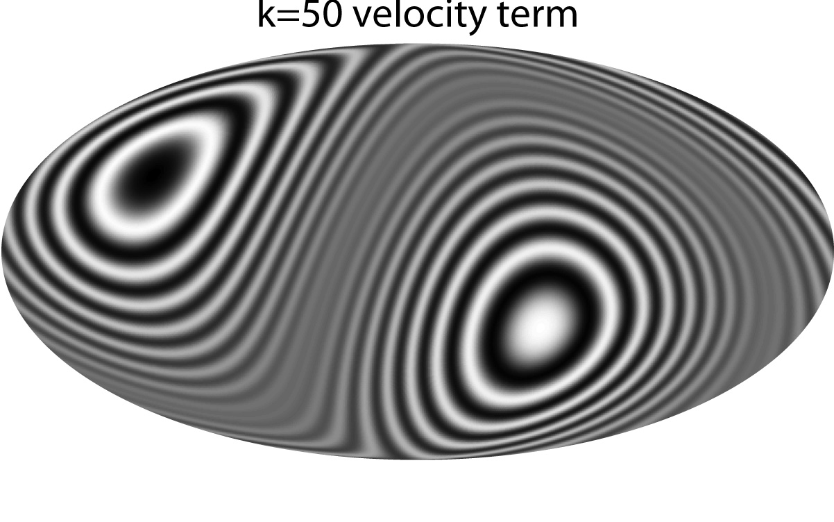Figure 1.3. Left: The scalar density and potential perturbation. Right: The vector velocity perturbation.

The anisotropy is usually expanded in spherical harmonics:

(1.13)

Because the Universe is approximately isotropic the probability densities for all the different m's at a given are identical. Furthermore, the expected value of T() is obviously zero, and thus the expected values of the a _m's is zero. But the variance of the a _m's is a measurable function of , defined as

(1.14)

Note that in this normalization C and a _m are dimensionless. The harmonic index associated with an angular scale is given by 180° / , but the total number of spherical harmonics contributing to the anisotropy power at angular scale is given by times 2 + 1. Thus to have equal power on all scales one needs to have approximately C ^-2. Given that the square of the angular momentum operator is actually ( + 1), it is not surprising that the actual angular power spectrum of the CMB predicted by "equal power on all scales" is

(1.15)

where < Q² > or Q²_rms-PS is the expected variance of the = 2 component of the sky, which must be divided by T₀² because the a _m's are defined to be dimensionless. The "4" term arises because the mean of |Y _m|² is 1 / (4), so the |a _m|²'s must be 4 times larger to compensate. Finally, the quadrupole has 5 components, while C is the variance of a single component, giving the "5" in the denominator. The COBE DMR experiment determined (< Q² >)^1/2 = 18 µK, and that the C's from = 2 to = 20 were consistent with Equation 1.15.

The other common way of describing the anisotropy is in terms of

(1.16)

Note these definitions give T₂² = 2.4 < Q² >. Therefore, the COBE normalized Harrison-Zel'dovich spectrum has T² = 2.4 × 18² = 778 µK² for 20.

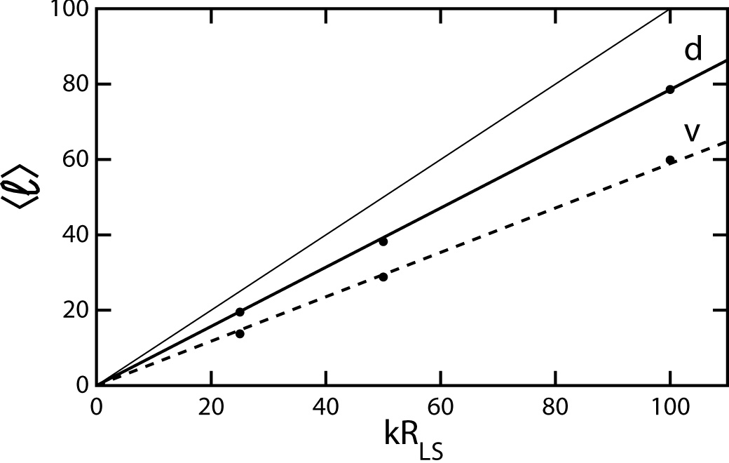
It is important to realize that the relationship between the wavenumber k and the spherical harmonic index is not a simple = k R_LS. Figure 1.3 shows that while = k R_LS at the "equator" the poles have lower . In fact, if µ = cos, where is the angle between the wave vector and the line-of-sight, then the "local " is given by k R_LS (1 - µ²)^1/2. The average of this over the sphere is < > = ( / 4) k R_LS. For the velocity term the power goes to zero when µ = 0 on the equator, so the average is smaller, < > = (3 / 16) k R_LS, and the distribution of power over lacks the sharp cusp at = k R_LS. As a result the velocity term, while contributing about 60% as much to the RMS anisotropy as the density term, does not contribute this much to the peak structure in the angular power spectrum. Thus the old nomenclature of "Doppler" peaks was not appropriate, and the new usage of "acoustic" peaks is more correct. Figure 1.4 shows the angular power spectrum from single k skies for both the density and velocity terms for several values of k, and a graph of the variance-weighted mean vs. kR_LS. These curves were computed numerically but have the expected forms given by the spherical Bessel function j for the density term and j' for the velocity term.

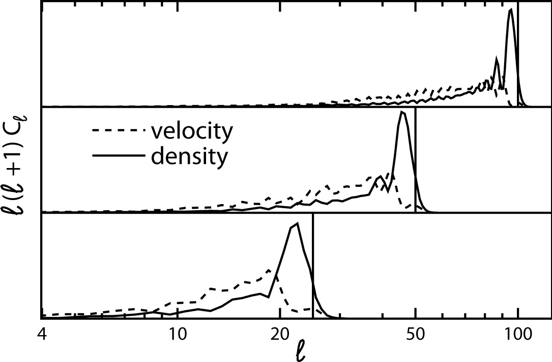Figure 1.4. Left: Mean is plotted vs. the wavenumber kRLS. The light solid line shows = kRLS, while the solid line shows = ( / 4)kRLS, and the dashed line shows = (3 / 16)kRLS. Right: The angular power spectra for single k skies is plotted for kRLS = 25, 50, and 100 (from bottom to top).

Seljak (1994) considered a simple model in which the photons and baryons are locked together before recombination, and completely noninteracting after recombination. Thus the opacity went from infinity to zero instantaneously. Prior to recombination there were two fluids, the photon-baryon fluid and the CDM fluid, which interacted only gravitationally. The baryon-photon fluid has a sound speed of about c / 3^1/2 while the dark matter fluid has a sound speed of zero. Figure 1.5 shows a conformal spacetime diagrams with a traveling wave in the baryon-photon fluid and the stationary wave in the CDM. The CDM dominates the potential, so the large-scale structure (LSS) forms in the potential wells defined by the CDM.

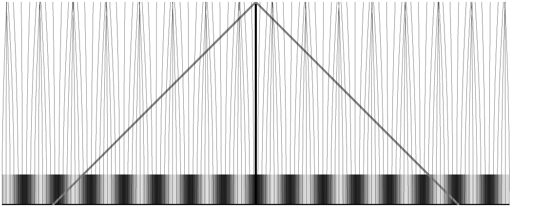Figure 1.5. On the left a conformal spacetime diagram showing a traveling wave in the baryon-photon fluid. On the right, the stationary CDM wave and the world lines of matter falling into the potential wells. For this wavenumber the density contrast in the baryon-photon fluid has undergone one-half cycle of its oscillation and is thus in phase with the Sachs-Wolfe effect from the CDM. This condition defines the first acoustic peak.

In Seljak's simple two-fluid model, there are five variables to follow: the density contrast in the CDM and baryons, _c and _b, the velocities of these fluids _c and _b, and the potential . The photon density contrast is (4/3)_b. In Figure 1.6 the density contrasts are plotted vs. the scale factor for several values of the wavenumber. To make this plot the density contrasts were adjusted for the effect of the potential on the time, with

(1.17)

and

(1.18)

Remembering that is negative when is positive, the two terms on the right-hand side of the above equations cancel almost entirely at early times, leaving a small residual growing like a² prior to a_eq, the scale factor when the matter density and the radiation density were equal. Thus these adjusted density contrasts evolve like ^-1-1 in homogeneous universes.

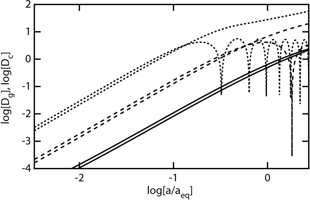Figure 1.6. Density contrasts in the CDM and the photons for wavenumbers = 5, 20, and 80 (see Fig. 1.7) as a function of the scale factor relative to the scale factor and when matter and radiation densities were equal. The photon density contrast starts out slightly larger than the CDM density contrast but oscillates.

Figure 1.7 shows the potential that survives to recombination and produces LSS, the potential plus density effect on the CMB temperature, and the velocity of the baryons as function of wavenumber. Close scrutiny of the potential curve in the plot shows the baryonic wiggles in the LSS that may be detectable in the large redshift surveys by the 2dF and SDSS groups.

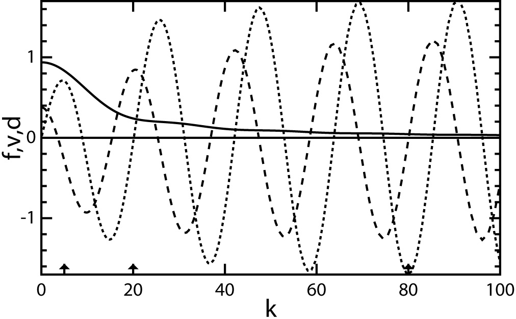Figure 1.7. Density contrasts at recombination as a function of wavenumber . The arrows on the x-axis indicate the values of for vs. a, as plotted in Figure 1.6. The solid curve shows the potential (the initial potential is always = 1), the long dashed curve curve shows the combined potential plus density effect on the CMB temperature, while the short dashed curve shows the velocity of the baryon-photon fluid.

A careful examination of the angular power spectrum allows several cosmological parameters to be derived. The baryon to photon ratio and the dark matter to baryon density ratio can both be derived from the amplitudes of the first two acoustic peaks. Since the photon density is known precisely, the peak amplitudes determine the baryon density _b = _b h² and the cold dark matter density _c = _CDM h². The matter density is given by _m = _b + _CDM. The amplitude < Q² > and spectral index n of the primordial density perturbations are also easily observed. Finally the angular scale of the peaks depends on the ratio of the angular size distance at recombination to the distance sound can travel before recombination. Since the speed of sound is close to c / 3^1/2, this sound travel distance is primarily affected by the age of the Universe at z = 1100. The age of the Universe goes like t ^-1/2 _m^-1/2 h^-1. The angular size distance is proportional to h^-1 as well, so the Hubble constant cancels out. The angular size distance is almost proportional to _m^-1/2, but this relation is not quite exact. Figure 1.8 compares the angular size distance to _m^-1/2. One sees that a peak position that corresponds to _tot = 0.95 if _m = 0.2 can also be fit by _tot = 1.1 if _m = 1. Thus, to first order the peak position is a good measure of _tot.

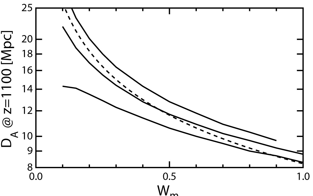Figure 1.8. The angular size distance vs. m for H0 = 60 km s-1 Mpc-1 and three different values of tot (0.9, 1, and 1.1, from top to bottom). The dashed curve shows m-1/2.

The CMBFAST code by Seljak & Zaldarriaga (1996) provides the ability to quickly compute the angular power spectrum C. Typically CMBFAST runs in about 1 minute for a given set of cosmological parameters. However, two different groups have developed even faster methods to evaluate C. Kaplinghat, Knox, & Skordis (2002) have published the Davis Anisotropy Shortcut (DASh), with code available for download. This program interpolates among precomputed C's. Kosowsky, Milosavljevic, & Jiminez (2002) discuss combinations of the parameters that produce simple changes in the power spectrum, and also allow accurate and fast interpolation between C's. These shortcuts allow the computation of a C from model parameters in about 1 second. This allows the rapid computation of the likelihood of a given data set D for a set of model parameters M, L(D|M). When computing the likelihood for high signal-to-noise ratio observations of a small area of the sky, biases due to the non-Gaussian shape of the likelihood are common. This can be avoided using the offset log-normal form for the likelihood L(C) advocated by Bond, Jaffe, & Knox (2000).

Table 1.1. Beam Size and Calibration Corrections

Experiment	b (')	100() /	100( dT) / dT
COBE	420.0	-0.3	...
ARCHEOPS	15.0	-0.2	2.7
BOOMERanG	12.9	10.5	-7.6
MAXIMA	10.0	-0.9	0.2
DASI	5.0	-0.4	0.7
VSA	3.0	-0.5	-1.7
CBI	1.5	-1.1	-0.2

Wright (1994) gave the example of determining the primordial power spectrum power-law index n, P(k) = A(k / k₀)ⁿ. Marginalizing over the amplitude by integrating the likelihood over A gives very different results for different values of k₀. Thus, it is very unfortunate that Hu & Dodelson (2002) still accept integration over the likelihood.

Instead of integrating over the likelihood one needs to define the a posteriori probability of the models p_f(M) based on an a priori distribution p_i(M) and Bayes' theorem:

(1.19)

It is allowable to integrate p_f over the space of models because the prior will transform when changing variables so as to keep the integral invariant.

In the modeling reported here, the a priori distribution is chosen to be uniform in _b, _c, n, _V, _tot, and z_ri. In doing the fits, the model C's are adjusted by a factor of exp[a + b ( + 1)] before comparison with the data. Here a is a calibration adjustment, and b is a beam size correction that assumes a Gaussian beam. For COBE, a is the overall amplitude scaling parameter instead of a calibration correction. Marginalization over the calibration and beam size corrections for each experiment, and the overall spectral amplitude, is done by maximizing the likelihood, not by integrating the likelihood. Table 1.1 gives these beam and calibration corrections for each experiments. All of these corrections are less than the quoted uncertainties for these experiments. BOOMERanG stands out in the table for having honestly reported its uncertainties: ± 11% for the beam size and ± 10% for the gain. The likelihood is given by

(1.20)

where j indexes over experiments, i indexes over points within each experiment, Z = ln(C + N) in the offset log normal approach of Bond et al. (2000), and N is the noise bias. Since for COBE a is the overall normalization, σ(a) is set to infinity for this term to eliminate it from the likelihood. The function f(x) is x² for small |x| but switches to 4(|x| - 1) when |x| > 2. This downweighs outliers in the data. Most of the experiments have double tabulated their data. I have used both the even and odd points in my fits, but I have multiplied the 's by 2^1/2 to compensate. Thus, I expect to get ² per degree of freedom close to 0.5 but should have the correct sensitivity to cosmic parameters.

Table 1.2. Cosmic Parameters from pre-WMAP CMB Data only

Parameter	Mean		Units
b	0.0206	0.0020
c	0.1343	0.0221
V	0.3947	0.2083
k	-0.0506	0.0560
zri	7.58	3.97
n	0.9409	0.0379
H0	51.78	12.26	km s-1 Mpc-1
t0	15.34	1.60	Gyr
	0.2600	0.0498

The scientific results such as the mean values and the covariance matrix of the parameters can be determined by integrations over parameter space weighted by p_f. Table 1.2 shows the mean and standard deviation of the parameters determined by integrating over the a posteriori probability distribution of the models. The evaluation of integrals over multi-dimensional spaces can require a large number of function evaluations when the dimensionality of the model space is large, so a Monte Carlo approach can be used. To achieve an accuracy of () in a Monte Carlo integration requires (^-2) function evaluations, while achieving the same accuracy with a gridding approach requires (^-n/2) evaluations when second-order methods are applied on each axis. The Monte Carlo approach is more efficient for more than four dimensions. When the CMB data get better, the likelihood gets more and more sharply peaked as a function of the parameters, so a Gaussian approximation to L(M) becomes more accurate, and concerns about banana-shaped confidence intervals and long tails in the likelihood are reduced. The Monte Carlo Markov Chain (MCMC) approach using the Metropolis-Hastings algorithm to generate models drawn from p_f is a relatively fast way to evaluate these integrals (Lewis & Bridle 2002). In the MCMC, a "trial" set of parameters is sampled from the proposal density p_t(P';P), where P is the current location in parameter space, and P' is the new location. Then the trial location is accepted with a probability given by

(1.21)

When a trial is accepted the Markov chain one sets P = P'. This algorithm guarantees that the accepted points in parameter space are sampled from the a posteriori probability distribution.

The most common choice for the proposal density is one that depends only on the parameter change P'- P. If the proposal density is a symmetric function then the ratio p_t(P;P') / p_tP';P) = 1 and is then just the ratio of a posteriori probabilities. But the most efficient choice for the proposal density is p_f(P) which is not a function of the parameter change, because this choice makes = 1 and all trials are accepted. However, if one knew how to sample models from p_f, why waste time calculating the likelihoods?

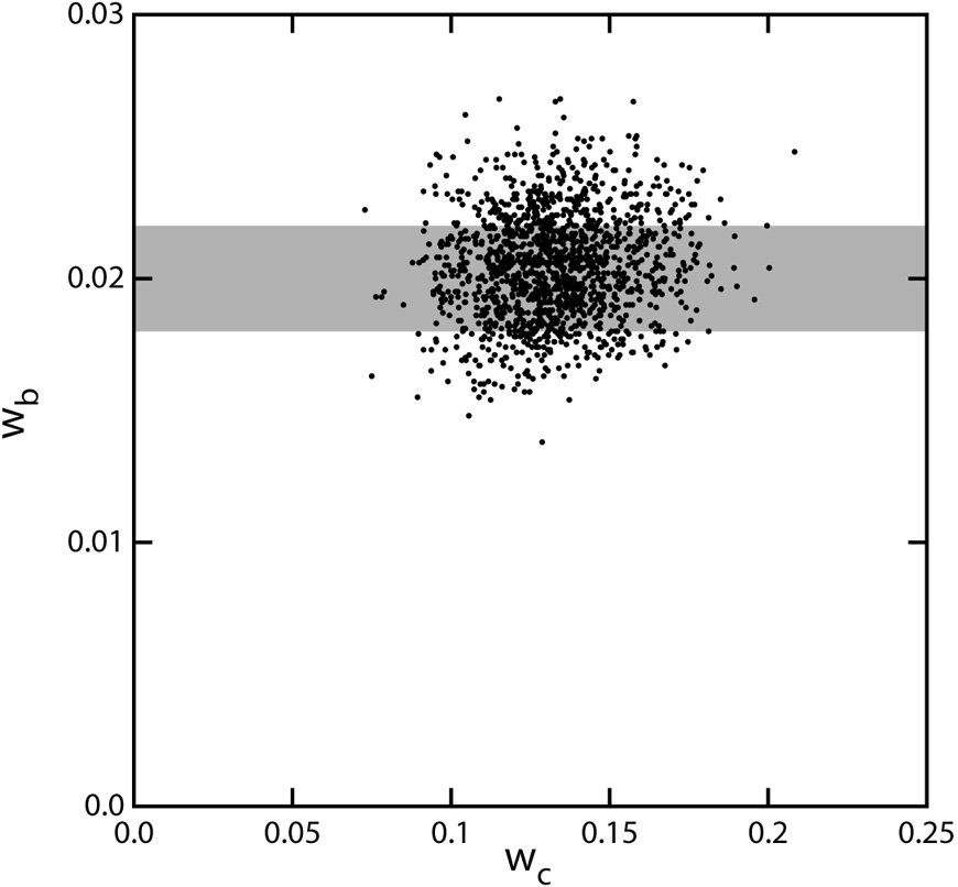
Just plotting the cloud of points from MCMC gives a useful indication of the allowable parameter ranges that are consistent with the data. I have done some MCMC calculations using the DASh (Kaplinghat et al. 2002) to find the C's. I found DASh to be user unfriendly and too likely to terminate instead of reporting an error for out-of-bounds parameter sets, but it was fast. Figure 1.9 shows the range of baryon and CDM densities consistent with the CMB data set from COBE (Bennett et al. 1996), ARCHEOPS (Amblard 2003), BOOMERanG (Netterfield et al. 2002), MAXIMA (Lee et al. 2001), DASI (Halverson et al. 2002), VSA (Scott et al. 2003), and CBI (Pearson et al. 2003), and the range of matter and vacuum densities consistent with these data. The Hubble constant is strongly correlated with position on this diagram. Figure 1.10 shows the distribution of t₀ for models consistent with this pre-WMAP CMB data set. The relative uncertainty in t₀ is much smaller than the relative uncertainty in H₀ because the low-H₀ models have low vacuum energy density (_V), and thus low values of the product H₀ t₀. The CMB data are giving a reasonable value for t₀ without using information on the distances or ages of objects, which is an interesting confirmation of the Big Bang model.

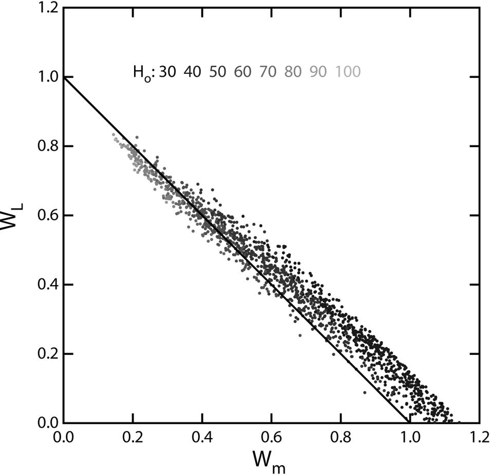Figure 1.9. Left: Clouds of models drawn from the a posteriori distribution based on the CMB data set as of 19 November 2002. The gray band shows the Big Bang nucleosynthesis determination of b (± 2) from Burles, Nollett, & Turner (2001). Right: the same set of models in the m, plane.

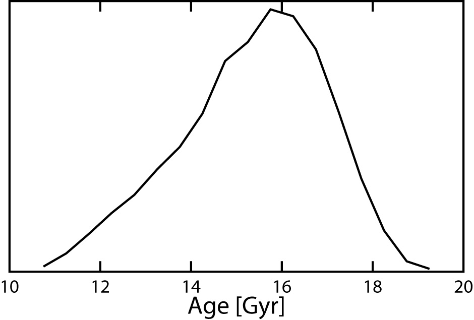Figure 1.10. Distribution of the age of the Universe based only on the pre-WMAP CMB data.

Peacock & Dodds (1994) define a shape parameter for the observed LSS power spectrum, = _m h exp(-2_b). There are other slightly different definitions of in use, but this will be used consistently here. Peacock & Dodds determine = 0.255 ± 0.017 + 0.32(n^-1-1). The CMB data specify n, so the slope correction in the last term is only 0.020 ± 0.013. Hence, the LSS power spectrum wants = 0.275 ± 0.02. The models based only on the pre-WMAP CMB data give the distribution in shown in Figure 1.11, which is clearly consistent with the LSS data.

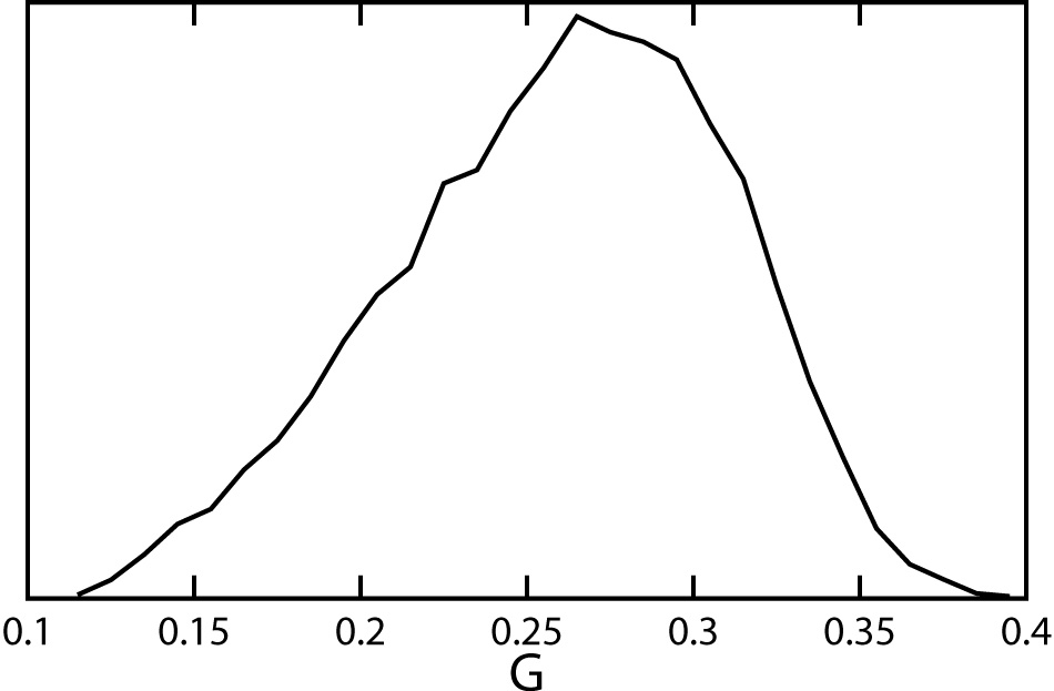Figure 1.11. Distribution of the LSS power spectrum shape parameter = m h exp(-2b) from the pre-WMAP CMB data.

Two examples of flat (_tot = 1) models with equal power on all scales (n = 1), plotted on the pre-WMAP data set, are shown in Figure 1.12. Both these models are acceptable fits, but the CDM model is somewhat favored based on the positions of the peaks. The rise in C at low for the CDM model is caused by the late integrated Sachs-Wolfe effect, which is due to the changing potential that occurs for z < 1 in this model. The potential changes because the density contrast stops growing when dominates while the Universe continues to expand at an accelerating rate. The potential change during a photon's passage through a structure produces a temperature change given by T / T = 2 / c² (Fig. 1.13). The factor of 2 is the same factor of 2 that enters into the gravitational deflection of starlight by the Sun. The effect should be correlated with LSS that we can see at z 0.6. Boughn & Crittenden (2003) have looked for this correlation using COBE maps compared to radio source count maps from the NVSS, and Boughn, Crittenden, & Koehrsen (2002) have looked at the correlation of COBE and the X-ray background. As of now the correlation has not been seen, which is an area of concern for CDM, since the (non)correlation implies = 0 ± 0.33 with roughly Gaussian errors. This correlation should arise primarily from redshifts near z = 0.6, as shown in Figure 1.14. The coming availability of LSS maps based on deep all-sky infrared surveys (Maller 2003) should allow a better search for this correlation.

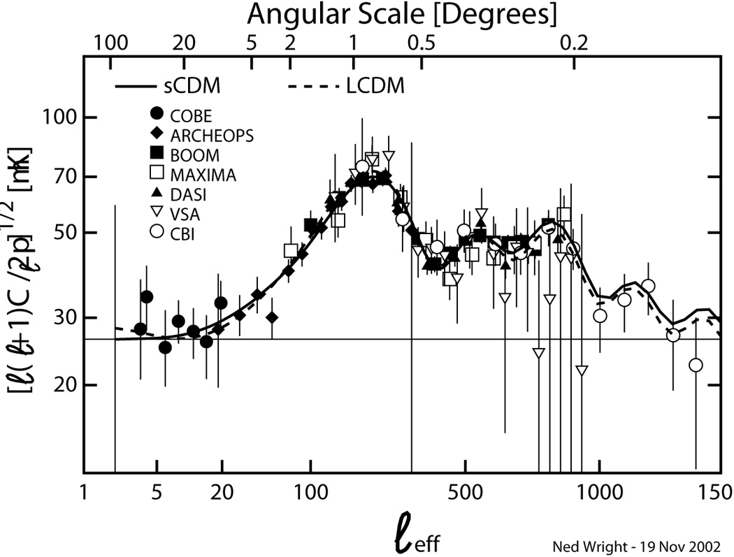Figure 1.12. Two flat n = 1 models. One shows CDM with = 2/3. The best fit gives b = 0.022 and c = 0.132, implying H0 = 68 km s-1 Mpc-1. The other fit shows = 0 with b = 0.021 and c = 0.196, implying H0 = 47 km s-1 Mpc-1.

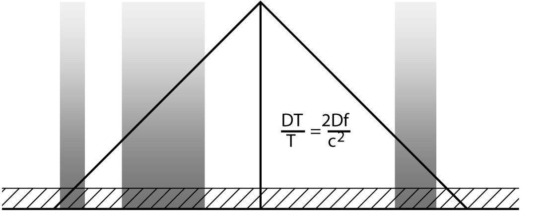Figure 1.13. Fading potentials cause large-scale anisotropy correlated with LSS due to the late integrated Sachs-Wolfe effect.

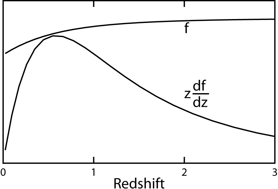Figure 1.14. Change of potential vs. redshift in a CDM model. Note that the most significant changes occur near z = 0.6.

In addition to the late integrated Sachs-Wolfe effect from , reionization should also enhance C at low , as would an admixture of tensor waves. Since , _ri and T / S all increase C at low , and this increase is not seen, one has an upper limit on a weighted sum of all these parameters. If is finally detected by the correlation between improved CMB and LSS maps, or if a substantial _ri, such as the = 0.1 predicted by Cen (2003), is detected by the correlation between the E-mode polarization and the anisotropy (Zaldarriaga 2003), then one gets a greatly strengthened limit on tensor waves.