Annu. Rev. Astron. Astrophys. 1988. 26: 561-630 Copyright © 1988 by Annual Reviews. All rights reserved

6.2. The Hubble Diagram at Large Redshifts

Determination of the second term involving q₀ in Equations 33-35 was the principal motivation for extending the Hubble m(z) diagram to the largest possible redshifts. The correction is of first order in z (cf. Equation 34) and hence is a large effect. To see how large, recall the special cases of q₀ = 0 and q₀ = 1/2 for Rr₀ of Equations 22 and 26, which (when put into Equation 32 for the flux) give the closed expressions

(41)

and

(42)

where the constant is the same in both equations. These are special cases of the general equation (Equation 33). If, then, we could observe to z = 1 and determine m_bol, the magnitude difference between the q₀ = 0 and q₀ = 1/2 cases would be m_bol = 0.54 mag, the q₀ = 1/2 case being brighter, assuming no luminosity evolution in the look-back time.

Early studies aimed to determine q₀ this way were reviewed by Peach (1970, 1972). Special programs to extend the Hubble diagram to very large redshifts were begun by Gunn & Oke (1975), Sandage et al. (1976), Kristian et al. (1978), Hoessel (1980), and Schneider et al. (1983a, b), and these studies reached redshifts of z = 0.5 (excluding the radio galaxies). Very much larger redshifts for cluster galaxies have become available by including radio sources in the sample [see Spinrad (1986, and references therein) for a review].

6.2.1 CORRECTIONS TO THE MAGNITUDES FOR THE HUBBLE DIAGRAM   Several technical corrections are needed before Equation 35 can be used to obtain q₀.

1. The aperture correction must be made to reduce the photometric measurements to either a standard isophote (Sandage 1975a, Table B1) or to a standard metric diameter (Sandage 1972a, Table 3). The first method requires knowledge of the isophotal radius such as that of Holmberg (1958), or the D_s of HMS (appendix A) estimated from the original Palomar Sky Survey blue plates, or D(0) of de Vaucouleurs et al. (1977; hereinafter RC2). The argument of the generally adopted standard curve (Sandage 1975a, Table B1) is / 2.5D(0). The second method, using a standard metric diameter, depends on q₀, because the space curvature is needed to calculate the r(z) function (Equations 29 and 30 of Section 3.1), but the q₀ dependence of the final magnitude correction is nearly negligible, provided that the chosen standard radius is large enough. This is shown by the metric aperture corrections calculated by Kristian et al. (1978) for q₀ = 0 and q₀ = + 1 separately. The final magnitudes differ by less than 0.1 mag between the two q₀ models, even for z = 0.5, belying the criticism of Segal (1976) concerning a circular argument that he implies leads to a lack of convergence of the method and therefore to an incorrect conclusion concerning the linearity of the velocity field.

Gunn & Oke (1975) use the same precept for their aperture corrections by reducing their data to a standard aperture that corresponds to a metric radius of ~ 16 kpc (for H₀ = 60, q₀ = 1/2). That of Sandage is at ~ 86 kpc (H₀ = 50). The Oke-Gunn radius is so small, however, that the dependence of their aperture corrections on q₀, done this way, is much larger than for the correction used by Sandage (1975a) and by Kristian et al. (1978).

2. Galactic absorption corrections are controversial, depending on the assumption of either large (de Vaucouleurs & Malik 1969) or near-zero (Sandage 1972b, Section III) absorption at the Galactic pole. Galaxy counts have always been interpreted as requiring absorption at the pole, even as high as A_B ~ 0.5 mag (Hubble 1934, Shane & Wirtanen 1954, 1967, Noonan 1971, Holmberg 1974, Heiles 1976), but Noonan makes the point that counts below b = 45° need not be related to counts at the pole if the Galactic absorption is patchy [small clouds, such as scattered summer cumulus, with which the zenith is mostly clear but the horizon is not due to the highly nonlinear areas (on the sky) at equal intervals of the zenith angle intervals].

The absorption-free polar cap model of McClure & Crawford (1971) is consistent with galaxy colors as a function of latitude (Sandage 1973a, Sandage & Visvanathan 1978, Section VI), leading to the absorption correction of A_B = 0.13(csc b - 1) for |b| < 50° and A_B = 0 for |b| > 60°, but smoothed for |b| = 50 - 60° to avoid a step. This correction was used in the Mount Wilson series of papers on the m(z) Hubble diagram mentioned in Section 6.1.2.

3. A cluster richness correction has been derived by correlating the population of clusters with the magnitude deviations of individual first-ranked cluster galaxies from the m(z) ridge line. Early indications that the change in M_v (brightest) with cluster richness was negligible at the ± 0.1 mag level (Peach 1969, Sandage 1972b, his Figure 8) had to be modified when a prior correction was made for contrast effect (Section 6.2.2); this correction gave a measurable trend of M_v with a range of 0.4 mag over the Abell richness classes from 0 to 4 (Sandage & Hardy 1973). More complete data (Sandage et al. 1976, their Figure 3; Schneider et al. 1983b, their Figure 3) reduce the amplitude of the effect for first-ranked galaxies to ~ 0.3 mag over the same richness range. This is so small as to keep the problem unsolved as to whether the M = f (richness) data are consistent with (a) a stochastic sampling of the luminosity function or (b) special formation conditions of brightest cluster galaxies. A large literature exists on each side of the issue. Early papers by Peebles (1968, 1969), Peach (1969), and Peterson (1970a, b) came to different conclusions. New data on sparse groups (Sandage 1976), when combined with all existing data on great clusters, showed that the variation of the absolute magnitudes of first-, second-, and third-ranked cluster galaxies with richness was too shallow to be explained by the bright-end slope to (M). The opposite conclusion was stated by Geller & Peebles (1976), although their calculations clearly do not fit the data (their Figure 9). Schechter & Peebles (1976), admitting this, then attributed the lack of agreement between a statistical theory and the data to a Malmquist-like selection effect if the sparse groups were chosen from flux-limited catalogs. Nevertheless, their Figure 5 is an important one for practical cosmology, showing that the richness correction is, in fact, small for rich clusters (log N_c⁴⁸ > 1.4). This makes the observed correction (Sandage et al. 1976, their Figure 3) valid, even neglecting the supposed bias that results from using flux-limited samples.

The discussion took on new life with Tremaine & Richstone's (1977) conclusions from the data on the first three ranked galaxies that the special formation condition is marginally favored over the statistical theory. Geller & Postman (1983) concluded the opposite. Hence, the explanation of the M_i = f(richness) correlation appears not yet to be satisfactory. New data are needed on sparse groups, chosen from fainter flux-limited catalogs than those used by Sandage (1975a) or by Huchra & Geller (1982) and Geller & Huchra (1983). Despite this, as just mentioned, the richness correlation for the rich clusters, as determined directly from the observations [by either Sandage et al. (1976) or Schneider et al. (1983b)], does give a quite adequate correction of magnitudes to a standard cluster richness.

4. Bautz & Morgan (1970) devised a classification system for clusters and groups of galaxies based on the contrast in brightness of the first-ranked member with fainter cluster members. From a study of magnitude residuals about the mean m(z) ridge line, Sandage & Hardy (1973, their Figure 2) found that the absolute magnitude of the first-ranked galaxy correlated with Bautz-Morgan cluster type - the greater the contrast, the brighter M₁. A frequent explanation is that "cannibalism" of the first-ranked galaxy on its cluster family has occurred (Ostriker & Tremaine 1975, Ostriker & Hausman 1977, Hausman & Ostriker 1978, Tremaine 1981). Whatever its explanation, the contrast effect seems quite real for first-ranked galaxies. The amplitude of the correction determined by Schneider et al. (1983b, their Figure 3) is similar to that found earlier by Sandage & Hardy (1973, their Figure 2) and is well determined.

The four corrections just discussed (aperture, galactic absorption, richness, contrast), together with the K redshift dimming (Section 4.2), give the luminosity data needed for Equation 35 when applied to the measured magnitudes of first-ranked galaxies. The resulting m(z) Hubble diagram, plotted with the evolution effect E(z) taken to be zero, is reproduced here as Figure 5, taken from Sandage & Hardy (1973).

Figure 5. The m(z) fully corrected Hubble diagram for first-ranked E galaxies in clusters. Corrections to magnitudes are made for K dimming, absorption due to the Galaxy, the Bautz-Morgan contrast effect, and cluster richness (from Sandage & Hardy 1973).

The line in Figure 5 has the theoretical slope of 5 required by a linear redshift-distance relation. The scatter about this line is not a function of redshift. It has M₁) = 0.28 mag as the intrinsic dispersion of first-ranked cluster galaxies using "fully corrected" magnitudes, showing that such galaxies are among the best standard candles known as distance indicators.

6.2.2 ATTEMPTS TO DETERMINE q₀ IN OPTICAL WAVELENGTHS   In order to exploit the standard candle nature of first-ranked cluster galaxies, attempts have been made to determine q₀ from Equation 35 by (a) obtaining data to very large redshifts and (b) estimating the evolutionary correction E(t) from stellar evolution theory of the changing HR diagram with time, already described. The two early attempts using the Hubble diagram in optical wavelengths by Gunn & Oke (1975) and by Sandage et al. 1976) and Kristian et al. (1978) (discussed earlier) reached only z = 0.75, which, from Equations 39 and 40, gives a wedge of only mag = 0.4 mag on the problem between the q₀ = 0 and q₀ = 1/2 cases. Because of the smallness of the effect to this small limiting redshift, it is not so surprising that the formal solutions given by the two groups of q₀ = 0.33 ± 0.7 or q₀ = - 1.27 ± 0.7 by Gunn & Oke and q₀ = 1.6 ± 0.4 by Kristian et al. (and later q₀ = -0.55 ± 0.45 by Hoessel et al. 1980) are as close as they are. Furthermore, the solutions mean nothing until the E(t) correction for luminosity evolution is applied. This term is large in BVR wavelengths. Because it is expected to be small in the near-IR, major studies were begun in the early 1980s in this wavelength region.

6.2.3. THE HUBBLE DIAGRAM   The two principal advantages of observations in the near-IR for large redshifts are (a) that the K correction is appreciably smaller than in the B and V wavelengths, and (b) that the E(t) evolution term is insensitive to starburst evolution (termed active evolution by Lilly & Longair 1984). Furthermore, its amplitude for passive evolution (i.e. the gradual evolution of the HR diagram of an old coveal population with time) is also much smaller in the K band than in the UBV or R bands.

A pioneering advance in K-band photometry was made by Grasdalen (1980) and by Lebofsky (1980), who gave the first m(z) Hubble IR diagram. Lebofsky (1981), by including radio galaxies, reached z = 1.18 and obtained a value of q₀ = 0.05 ± 0.30 for z < 0.5, where the E_K(t) evolution term was taken to be zero. A hint for mild evolution for z > 0.5 was found even in these early data. More extensive observations (Lebofsky & Eisenhardt 1986) continued to show evidence for mild luminosity evolution, consistent with Tinsley's (1978) predictions.

Lilly & Longair (1982, 1984) greatly extended the sample using radio galaxies, reaching z > 1 with a substantial number of objects. They concluded that q₀ ~ 0.5 if E_K(z = 1) = 1 mag, obtained from the (apparent) value of q₀ = 3.7 (their Figure 8). They countered a criticism concerning the use of radio galaxies for their survey by showing no difference in the m(z) relation between strong radio sources (using 3C sources, and hence with radio flux greater than 9 janskys) and weaker 1-jansky sources (Lilly et al. 1985).

These near-IR data gave the first convincing evidence for luminosity evolution in the look-back time to z = 1. A summary of the K data, with the m(z, E) model lines superposed, is given by Yoshii & Takahara (1988, their Figure 4), shown here as Figure 6. The conclusion from these data is that no model with E = 0 for q₀ < 1 fits the near-IR Hubble diagram data, and therefore that evolution is required, taking the data as they stand.

Figure 6. The near-IR Hubble m(z) diagram using K-band magnitudes corrected to a "standard metric" aperture size. The three left-hand theoretical curves are the expected relations (Equation 35) for q0 = 1.0 and q0 = 0.5 using the relevant E(t) evolution corrections. The redshift of galaxy formation is marked (z = 3,5, and 5). The three right-hand curves are for the marked q0 values with no evolution correction. K redshift corrections have been applied to the theoretical curves rather than the magnitudes (from Yoshii & Takahara 1988).

6.2.4 EVIDENCE FOR LUMINOSITY EVOLUTION FROM THE V-BAND HUBBLE DIAGRAM   Even more powerful evidence that the evolution term E(z) has been detected comes from the work at very large redshifts by Djorgovski et al. (1985), summarized by Spinrad (1986) and by Spinrad & Djorgovski (1987) using radio galaxies, reaching z = 1.8. Figure 7 is their summary Hubble diagram in V, in which data from a number of authors are combined. The V magnitudes are as observed, corrected only for aperture effect (no K correction). Theoretical lines from Equation 35 are shown [a K term and E(t) evolution according to various Bruzual models are put into the theoretical model lines, rather than corrections to the observations]. The conclusion is that the data for z > 0.8 cannot be fit by any q₀ value in the no-evolution case [i.e. E(t) = 0], whereas a good fit is obtained with a Bruzual evolving model with q₀ = 0 and H₀ = 50.

Figure 7. The m(z) Hubble diagram (plotted differently from Figure 5, with V magnitude as ordinate and linearly with z) extended to large redshift. Predicted theoretical m(z) lines for various q0 values and evolutionary corrections (Bruzual models) are shown. The K corrections have been applied to the theoretical curves (from Djorgovski et al. 1985).

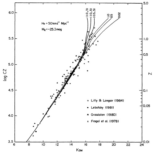
A different representation of a subset of these data is shown in Figure 8, again taken from Yoshii & Takahara (1988, their Figure 3). As before, the V magnitude is corrected only to the standard metric size for aperture effect. Again the K redshift dimming and E(t) corrections are put into the theoretical lines that show q₀ and the redshift of galaxy formation in the evolving models; these are shown as the four heavy lines to the left (H₀ = 50 km s^-1 Mpc^-1 is assumed so as to set the time scale of the evolution in the look-back time). The three lighter lines to the right are for no evolution for the q₀ = 1, 0.5, and 0.02 cases, none of which fit the data for z > 0.5. The assumed E(t) evolution, as explained earlier, is that given in Figure 2 of Yoshii & Takahara (1988), based on work by Arimoto & Yoshii (1986, 1987).

Figure 8. Same as Figure 6, but for V-band magnitudes (summary diagram from Yoshii & Takahara 1988).

The conclusion from Figures 7 and 8 is that evolution must be invoked if the prediction of the standard model (Equation 35) is to be claimed to be verified. This is a second demonstration (the first being the observed excess number counts over the predictions in Figures 3 and 4) that the observations cannot be used to confirm the simplest standard model because we must "save the phenomenon" by adding evolution. Of course, evolution is expected and, indeed, must be found if the standard model is to be correct because the mean age of the galaxies is required to be a function of redshift. However, it is important to note that the argument is circular if we use the standard model predictions to prove that evolution has occurred without having a priori proof that the standard model is correct. It is, then, incumbent on the claimer to show a consistent series of needs for look-back time evolution, independent of the N(m) and m(z) theoretical relations that themselves depend on the standard model. Stated differently, "The standard model requires evolution; and indeed, if evolution is left out, the model doesn't [and shouldn't] fit the data. On the other hand, to test the model with evolution we'd need an independent theory of the effects of evolution, which we don't yet have" (D. Layzer, private communication, 1988).