


In many cases the likelihood function is not analytical
or else, if analytical, the procedure for finding the
 j* and
the errors is too cumbersome and time consuming compared to
numerical methods using modern computers.
j* and
the errors is too cumbersome and time consuming compared to
numerical methods using modern computers.
For reasons of clarity we shall first discuss an inefficient, cumbersome method called the grid method. After such an introduction we shall be equipped to go on to a more efficient and practical method called the method of steepest descent.
The grid method
If there are M parameters
1, ... ,
M to be
determined one
could in principle map out a fine grid in M-dimensional space
evaluating w() (or
S()) at each
point. The maximum value
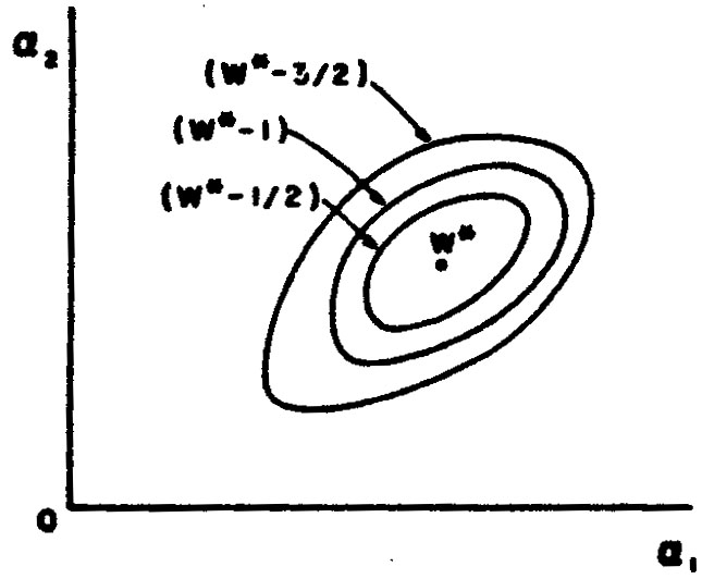
obtained for w is the maximum likelihood solution w*. One
could then map out contour surfaces of
w = (w* - ½), (w* - 1), etc. This
is illustrated for M = 2 in Fig. 6.
|
Figure 6. Contours of fixed w enclosing the max. likelihood solution w*. |
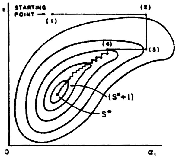
In the case of good statistics the contours would be small ellipsoids. Fig. 7 illustrates a case of poor statistics.

|
Figure 7. A poor statistics case of Fig. 6. |
Here it is better to present the (w* - ½) contour
surface (or the
(S* + 1) surface) than to try to quote errors on
. If
one is to quote errors it should be in the form
1-
< 1 <
1+
where
1- and
1+ are
the extreme excursions the surface makes
in 1 (see
Fig. 7). It could be a serious mistake to quote
a- or a+ as the errors in
1.
In the case of good statistics the second derivatives
ð2w /
ða
ðb = -
Hab could be found numerically in the region near
w*. The errors in the
's are then found by
inverting the H-matrix to obtain the error matrix for
; i.e.,
 = (H-1)ij. The second derivatives can be found
numerically by using
= (H-1)ij. The second derivatives can be found
numerically by using
|
In the case of least squares use
Hij = ½ ðS /
ði
ðj .
So far we have for the sake of simplicity talked in terms
of evaluating w()
over a fine grid in M-dimensional space.
In most cases this would be much too time consuming. A rather
extensive methodology has been developed for finding maxima or
minima numerically. In this appendix we shall outline just one
such approach called the method of steepest descent. We shall
show how to find the least squares minimum of
S(). (This is
the same as finding a maximum in
w()).
Method of Steepest Descent
At first thought one might be tempted to vary
1 (keeping
the other 's fixed) until a
minimum is found. Then vary
2
(keeping the others fixed) until a mew minimum is found, and
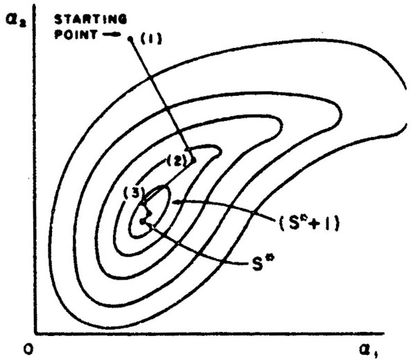
so on. This is illustrated in Fig. 8 where
M = 2 and the errors
are strongly correlated. But in Fig. 8 many
trials are needed.
This stepwise procedure does converge, but in the case of
Fig. 8, much too slowly. In the method of
steepest descent one moves against the gradient in
-space:
|
|
Figure 8. Contours of constant S
vs. |
So we change all the 's
simultaneously in the ratio ðS /
ð1 :
ðS /
ð2 :
ðS /
ð3 : ...
. In order to find the minimum along
this line in -space one
should use an efficient step size.
An effective method is to assume S(s) varies quadratically
from the minimum position s* where s is the distance along
this line. Then the step size to the minimum is
|
where S1, S2, and
S3 are equally spaced evaluations of
S(s) along s with step size
 s starting from
s1; i.e., s2 = s1
+ s,
s3 = s1 +
2s. One or two
iterations using the above formula will
reach the minimum along s shown as point (2) in
Fig. 9. The
next repetition of the above procedure takes us to point (3) in
Fig. 9. It is clear by comparing
Fig. 9 with Fig. 8 that the
method of steepest descent requires much fewer computer evaluations
of S() than does the
one variable at a time method.
s starting from
s1; i.e., s2 = s1
+ s,
s3 = s1 +
2s. One or two
iterations using the above formula will
reach the minimum along s shown as point (2) in
Fig. 9. The
next repetition of the above procedure takes us to point (3) in
Fig. 9. It is clear by comparing
Fig. 9 with Fig. 8 that the
method of steepest descent requires much fewer computer evaluations
of S() than does the
one variable at a time method.
|
Figure 9. Same as Fig. 8, but using the method of steepest descent. |
Least Squares with Constraints
In some problems the possible values of the
j are restricted
by subsidiary constraint relations. For example, consider
an elastic scattering event in a bubble chamber where the
measurements yj are track coordinates and the
i are track
directions and momenta. However, the combinations of
i that are
physically possible are restricted by energy-momentum conservation.
The most common way of handling this situation is to use the 4
constraint equations to eliminate 4 of the
's in
S(). Then S is
minimized with respect to the remaining
's. In this example
there would be (9 - 4) = 5 independent
's: two for orientation
of the scattering plane, one for direction of incoming track in
this plane, one for momentum of incoming track, and one for
scattering angle. There could also be constraint relations among
the measurable quantities yi. In either case, if the
method of
substitution is too cumbersome, one can use the method of Lagrange
multipliers.
In some cases the constraining relations are inequalities rather
than equations. For example, suppose it is known that
1 must be
a positive quantity. Then one could define a new set of
's where
(1')2 =
1,
2' =
2, etc. Now if
S(') is minimized no
non-physical values of a will be used in the search for the minimum.