5. MASS PRODUCTION OF TIME-DELAYS: H₀ WITH OTHER LENSES

Measuring time-delays has long been the main limitation to the use of quasar lenses in cosmology. Indeed, obtaining on a regular basis images of good quality and for long period of time is not easy. With the increasing number of large telescopes in excellent sites, and operated in "service mode", we have nevertheless entered a phase of mass production of time-delays. It took more than a decade to obtain the time-delay in Q 0957+561, but four time-delays were recently measured in one single thesis (Burud, 2000b) thanks to modern instrumentation and image deconvolution techniques. In addition, systematic imaging campaigns of lensed quasars such as the one carried out by CASTLE, facilitate the modeling of lens galaxies. Deep HST images are used in combination with spectroscopy, and along with what we know of the physics/dynamics of galaxies, to break the degeneracies between the models.

Even if the observational situation in quasar lensing is expected to improve a lot in the coming years, thanks to adaptive optics and 3D spectrographs, we can already say, with the precision of the observations collected so far, that lensed quasars are at least as powerful as other methods to determine H₀.

Let us play the naive game that consists in taking from literature the nine estimates of H₀, for each of the nine measured time-delays, and average them. This is summarized in Table 2 for all known lenses, along with the time-delay measurements. We indicate in the table the value obtained for H₀ with all kind of different models, just scaling the published errors to 1. Some authors consider isothermal spheres or ellipsoids with and without external shear. Others prefer to use lenses with constant mass-to-light ratios. In other words, the values we quote in Table 2 are all affected by unknown systematics. These systematics have been estimated by each author and included in the published error bars. If they had been under- or over- estimated, the dispersion between all the individual estimates of H₀, and the published errors on one single measurement, would be incompatible. Following our naive idea the averaged value for H₀, (without error weighting) is H₀ = 61 ± 7 km s^-1 Mpc^-1. Figure 12 is another way of displaying the data of Table 2, showing the value of H₀ as a function of the lens redshift. The 1 error region is dashed on the figure. Four measurements (in fact 3, if we include the mean value for the 2 estimates for HE 1104-1805 in the dashed area) are outside the 1 region, as expected for 9 independent measurements. Unless all the authors did the same systematic error (and this is unlikely because of the very different choices of models), the dispersion between the points is fully compatible with the individual error bars. This means that even if the models suffer from systematics, the amplitude of the error has been correctly estimated by the authors.

Table 2. Summary of measured time-delays, given with respect to the leading image. When several measurements have been obtained, we only give the more recent one. The 1 error as well as the relative error on the time-delay are given. The third column displays the value infered for H₀ for each system and the 1 error. In most cases we have considered the value given in the paper where the time-delay was published. When H₀ has been obtained by other authors, the reference is given as well.

Object	Time-delay(s)	H0
	(leading image first)	(km s-1 Mpc-1)
B 0218+357
Biggs et al. (1999)	(BA) = 10.5 ± 0.2 days (2%)	69+7-9
RX J0911+0551
Hjorth et al. (2002)	(BA) = 146 ± 4 days (3%)	71 ± 2 ( ± 4 syst)
Q 0957+561
Kundic et al. (1997)	(BA) = 417 ± 0.6 days (0.15%)	64 ± 7
	but multiple time-delays
Goicoechea (2002)	(BA) = 425 ± 4.0 days (1.0%)
	(BA) = 432 ± 1.9 days (0.5%)
HE 1104-1805	Strong micro/milli-lensing
Gil-Merino et al. (2002)	(AB) = 310 ± 9 days (3%)	48 ± 2 or 62 ± 2
PG 1115+080
Schechter et al. (1997)	(CB) = 25+3.3-3.8 days (14%)
Barkana (1997)	(CA) = 13 days
Treu & Koopmans (2002)		59 +12-7 ( ± 3 syst)
SBS 1520+53
Burud et al. (2002)	(BA) = 130 ± 3 days (3%)	51 ± 9
B 1600+434	Radio and optical time-delays
Koopmans et al. (2000)	(BA) = 47 ± 5 days (10%)	57+7-6
Burud et al. (2000)	(BA) = 51 ± 2 days (4%)	52+7-4
B 1608+656
Fassnacht et al. (2002)	(BA) = 31.5 ± 2 days (6%)	63 ± 15
	(BC) = 36.0 ± 2 days (6%)
	(BD) = 77.0 ± 3 days (4%)
PKS 1830-211		No estimate. Lens
Lovell et al. (1998)	(BA) = 26+4-5 days (17%)	may be multiple
HE 2149-2745
Burud et al. (2002b)	(BA) = 103 ± 12 days (11%)	65 ± 8
COMBINED		61 ± 7

A more correct approach is to impose that a given family of profiles is used to model the mass distribution of lenses in general, and to impose that H₀ should be the same everywhere in the Universe. This has been done so far by very few authors. Williams & Saha (2000), use two systems and their non-parametric models, to infer H₀ = 61 ± 11 km s^-1 Mpc^-1(1 error). Courbin et al. (2002) add two other lenses to the Williams & Saha sample, and adopt the same non-parametric technique to infer H₀ = 64 ± 4 km s^-1 Mpc^-1. Using parametric lens models and a set of 4 different lenses (only PG 1115+080 is common to all authors) Kochanek (2002) obtain H₀ = 51 ± 5 km s^-1 Mpc^-1if lens galaxies have dark matter halos, or H₀ = 73 ± 8 km s^-1 Mpc^-1 if lens galaxies have constant mass-to-light ratios.

Gravitationally lensed quasars have one drawback over other methods for determining H₀: they do require good knowledge of the mass profile of the lens. It has long been a limitation to the effectiveness of the method to produce reliable estimates of H₀, but this drawback is becoming easier and easier to overcome, thanks to spectroscopy, to high spatial resolution observations, and to the progresses made on the physics of galaxies. Gravitational lenses have, on the other hand, tremendous advantages over other methods. First, they do not rely on any "standard candle" which would rend the method close to useless if the standard candle turned out to be significantly deviant from the "standard" behaviour. Second, it does not require secondary calibrators of the standard candle, e.g., low redshift objects, in the case of the supernovae method. Third, it probes H₀ at cosmological distances, independent of any local effect such as peculiar velocities of nearby galaxies. Finally, lensing is not as sensitive to the other cosmological parameters (_m, ) than the other methods.

We compare in Fig. 12, the value of H₀ for lensed quasars and for the Cepheid method. With the present error bars, calculated with only 9 objects, we can say that lensed quasars and Cepheid disagree. Lensing gives lower values for H₀ than does the Cepheid method. If our knowledge of the mass distribution of galaxies is any good, i.e., that galaxies have dark matter halos, the lensing value would be even smaller. Recent CMB experiments such as WMAP find high values for H₀ (e.g., Spergel et al. 2003), in agreement with the local estimate: H₀ = 71, with impressive error bars of only 4%. With the high degree of degeneracy between the cosmological models used to represent the observed CMB power spectrum, H₀ is in fact shown to take any value between 54 and 72 (Efstathiou 2003). It spans over an even broader ranger if one does not invoke any prior knowledge on the value of _m and as determined with supernovae.

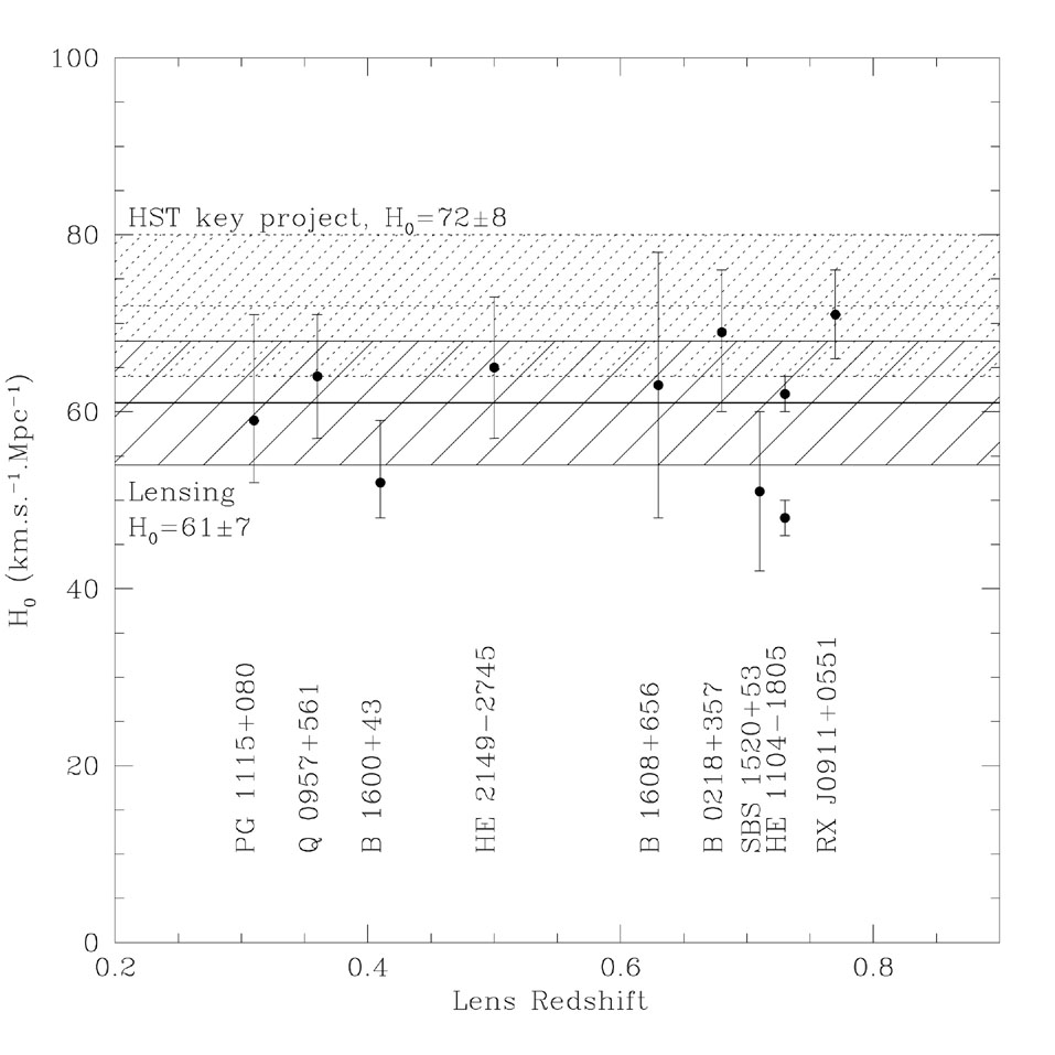Figure 12. Values of H0 for all lenses with known time-delays. H0 is given as a function of lens redshift, directly taken from the literature. The dashed area shows the range of possible values, according to lensing, which is to be compared with the dashed-dotted area, infered from the Cepheid method in the framework of the HST key project. As in the case of PG 1115+080, the mean value for H0 is very marginally compatible with the local estimate of the Hubble parameter.

In fact, no single method has been proved to be good enough that it can surpass the others. There are, however, methods that are better than others as pinning down some of the cosmological parameters and it has been emphasized many times (Bridle et al. 2003) that all methods should be combined in order to break the degeneracies inherent to one specific method. Gravitational lensing is one of these methods. It has advantages and drawbacks, but probably many more advantages than drawbacks given the present observational context.

Acknowledgements. The author wishes to thank Alain Smette and Pierre Magain for useful discussions. Frédéric Courbin is supported by the European Commission through a Marie Curie Individual Fellowship, under grant MCFI-2001-0242. The collaborative grant ECOS/CONICYT C00U05 between Chile and France is also gratefully acknowledged.