2.5. The nearest neighbour method

The nearest neighbour class of estimators represents an attempt to adapt the amount of smoothing to the `local' density of data. The degree of smoothing is controlled by an integer k, chosen to be considerably smaller than the sample size; typically k n^1/2. Define the distance d (x, y) between two points on the line to be |x - y| in the usual way, and for each t define

to be the distances, arranged in ascending order, from t to the points of the sample.

The kth nearest neighbour density estimate is then defined by

(2.3)

In order to understand this definition, suppose that the density at t is f (t). Then, of a sample of size n, one would expect about 2r n f (t) observations to fall in the interval [t - r, t + r] for each r > 0; see the discussion of the naive estimator in Section 2.3 above. Since, by definition, exactly k observations fall in the interval [t - d_k(t), t + d_k(t)], an estimate of the density at t may be obtained by putting

this can be rearranged to give the definition of the kth nearest neighbour estimate.

While the naive estimator is based on the number of observations falling in a box of fixed width centred at the point of interest, the nearest neighbour estimate is inversely proportional to the size of the box needed to contain a given number of observations. In the tails of the distribution, the distance d_k(t) will be larger than in the main part of the distribution, and so the problem of undersmoothing in the tails should be reduced.

Like the naive estimator, to which it is related, the nearest choice neighbour estimate as defined in (2.3) is not a smooth curve. The function d_k(t) can easily be seen to be continuous, but its derivative will have a discontinuity at every point of the form 1/2(X_(j) + X_(j+k)), where X_(j) are the order statistics of the sample. It follows at once from these remarks and from the definition that will be positive and continuous everywhere, but will have discontinuous derivative at all the same points as d_k. In contrast to the kernel estimate, the nearest neighbour estimate will not itself be a probability density, since it will not integrate to unity. For t less than the smallest data point, we will have d_k(t) = X_(n-k+1) and for t > X_(n) we will have d_k(t) = t - X_(n-k+1). Substituting into (2.3), it follows that _- (t)dt is infinite and that the tails of die away at rate t^-1, in other words extremely slowly. Thus the nearest neighbour estimate is unlikely to be appropriate if an estimate of the entire density is required. 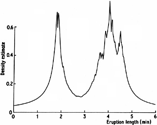Figure 2.10 gives a nearest neighbour density estimate for the Old Faithful data. The heavy tails and the discontinuities in the derivative are clear.

Fig. 2.10 Nearest neighbour estimate for Old Faithful geyser data, k = 20.

It is possible to generalize the nearest neighbour estimate to provide an estimate related to the kernel estimate. As in Section 2.4, let K(x) be a kernel function integrating to one. Then the generalized kth nearest neighbour estimate is defined by

(2.4)

It can be seen at once that (t) is precisely the kernel estimate evaluated at t with window width d_k(t). Thus the overall amount of smoothing is governed by the choice of the integer k, but the window width used at any particular point depends on the density of observations near that point.

The ordinary kth nearest neighbour estimate is the special case of (2.4) when K is the uniform kernel w of (2.1); thus (2.4) stands in the to same relation to (2.3) as the kernel estimator does to the naive ed. estimator. However, the derivative of the generalized nearest neighbour estimate will be discontinuous at all the points where the function d_k(t) has discontinuous derivative. The precise integrability and tail properties will depend on the exact form of the kernel, and to will not be discussed further here.

Further discussion of the nearest neighbour approach will be given in Section 5.2.