C. Inflation

1. The scenario

The deep issue inflation addresses is the origin of the large-scale homogeneity of the observable universe. In a relativistic model with positive pressure we can see distant galaxies that have not been in causal contact with each other since the singular start of expansion (Sec. II.C, Eq. [26]); they are said to be outside each other's particle horizon. Why do apparently causally unconnected parts of space look so similar? ⁽²⁶⁾ Sato (1981a, 1981b), Kazanas (1980), and Guth (1981) make the key point: if the early universe were dominated by the energy density of a relatively flat real scalar field (inflaton) potential V() that acts like , the particle horizon could spread beyond the universe we can see. This would allow for the possibility that microphysics during inflation could smooth inhomogeneities sufficiently to provide an explanation of the observed large-scale homogeneity. (We are unaware of a definitive demonstration of this idea, however.)

In the inflation scenario the field rolls down its potential until eventually V() steepens enough to terminate inflation. Energy in the scalar field is supposed to decay to matter and radiation, heralding the usual Big Bang expansion of the universe. With the modifications of Guth's (1981) scenario by Linde (1982) and Albrecht and Steinhardt (1982), the community quickly accepted this promising and elegant way to understand the origin of our homogeneous expanding universe. ⁽²⁷⁾

In Guth's (1981) picture the inflaton kinetic energy density is subdominant during inflation, ² << V(), so from Eqs. (30) the pressure p is very close to the negative of the mass density , and the expansion of the universe approximates the de Sitter solution, a exp(Ht) (Eq. [27]).

For our comments on the spectrum of mass density fluctuations produced by inflation and the properties of solutions of the dark energy models in Sec. III.E we will find it useful to have another scalar field model. Lucchin and Matarrese (1985a, 1985b) consider the potential

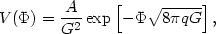(38)

where q and A are parameters. They show that the scale factor and the homogeneous part of the scalar field evolve in time as

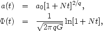(39)

where N = 2q( A)^1/2 / (G(6 - q))^1/2. If q < 2 this model inflates. Halliwell (1987) and Ratra and Peebles (1988) show that the solution (39) of the homogeneous equation of motion has the attractor property ⁽²⁸⁾ mentioned in connection with Eq. (31). This exponential potential is of historical interest: it provided the first clear illustration of an attractor solution. We return to this point in Sec. III.E.

A signal achievement of inflation is that it offers a theory for the origin of the departures from homogeneity. Inflation tremendously stretches length scales, so cosmologically significant lengths now correspond to extremely short lengths during inflation. On these tiny length scales quantum mechanics governs: the wavelenghts of zero-point field fluctuations generated during inflation are stretched by the inflationary expansion, ⁽²⁹⁾ and these fluctuations are converted to classical density fluctuations in the late time universe. ⁽³⁰⁾

The power spectrum of the fluctuations depends on the model for inflation. If the expansion rate during inflation is close to exponential (Eq. [27]), the zero-point fluctuations are frozen into primeval mass density fluctuations with power spectrum

(40)

Here (k, t) is the Fourier transform at wavenumber k of the mass density contrast (, t) = (, t) / <(t)> - 1, where is the mass density and <> the mean value. After inflation, but at very large redshifts, the spectrum in this model is P(k) k on all interesting length scales. This means the curvature fluctuations produced by the mass fluctuations diverge only as log k. The form P(k) k thus need not be cut off anywhere near observationally interesting lengths, and in this sense it is scale-invariant. ⁽³¹⁾ The transfer function T(k) accounts for the effects of radiation pressure and the dynamics of nonrelativistic matter on the evolution of (k, t), computed in linear perturbation theory, at redshifts z 10⁴. The constant A is determined by details of the chosen inflation model we need not get into.

The exponential potential model in Eq. (38) produces the power spectrum ⁽³²⁾

(41)

When n 1(q 0) the power spectrum is said to be tilted. This offers a parameter n to be adjusted to fit the observations of large-scale structure, though as we will discuss the simple scale-invariant case n = 1 is close to the best fit to the observations.

The mass fluctuations in these inflation models are said to be adiabatic, because they are what you get by adiabatically compressing or decompressing parts of an exactly homogeneous universe. This means the initial conditions for the mass distribution are described by one function of position, (, t). This function is a realization of a spatially stationary random Gaussian process, because it is frozen out of almost free quantum field fluctuations. Thus the single function of position is statistically prescribed by its power spectrum, as in Eqs. (40) and (41). More complicated models for inflation produce density fluctuations that are not Gaussian, or do not have simple power law spectra, or have parts that break adiabaticity, as gravitational waves (Rubakov, Sazhin, and Veryaskin, 1982) or magnetic fields (Turner and Widrow, 1988; Ratra, 1992b) or new hypothetical fields. All these extra features may be invoked to fit the observations, if needed. It may be significant that none seem to be needed to fit the main cosmological structure constraints we have now.

²⁶ Early discussions of this question are reviewed by Rindler (1956); more recent examples are Misner (1969), Dicke and Peebles (1979), and Zee (1980). Back.

²⁷ Aspects of the present state of the subject are reviewed by Guth (1997), Brandenberger (2001), and Lazarides (2002). Back.

²⁸ Ratra (1989, 1992a) shows that spatial inhomogeneities do not destroy this property, that is, for q < 2 the spatially inhomogeneous scalar field perturbation has no growing mode. Back.

²⁹ The strong curvature of spacetime during inflation makes the vacuum state quite different from that of Minkowski spacetime (Ratra 1985). This is somewhat analogous to how the Casimir metal plates modify the usual Minkowski spacetime vacuum state. Back.

³⁰ For the development of these ideas see Hawking (1982), Starobinsky (1982), Guth and Pi (1982), Bardeen, Steinhardt, and Turner (1983), and Fischler, Ratra, and Susskind (1985). Back.

³¹ The virtues of a spectrum that is scale-invariant in this sense were noted before inflation, by Harrison (1970), Peebles and Yu (1970), and Zel'dovich (1972). Back.

³² This is discussed by Abbott and Wise (1984), Lucchin and Matarrese (1985a, 1985b), and Ratra (1989, 1992a). Back.