4.2. Stellar Velocity Fields

The study of stellar velocity fields in galaxies is currently making very rapid progress. Almost all of the results discussed in this section are less than five years old. Many were made possible by the development of efficient detectors and image processing systems (cf. section 1). As a result, we are now able to ask incisive questions on the physics of galaxy structure and evolution.

Previous reviews of absorption-line kinematics have been published by Capaccioli (1979), Bertola (1981) and Illingworth (1981).

4.2.1. The Fourier Quotient Method

A number of efficient and impersonal methods have been developed for calculating stellar velocities and velocity dispersions using Fourier transform techniques. The advantages of these techniques, and basic machinery for their application are discussed in Brault and White (1971) and in Simkin (1974). In this paper I will discuss only the most widely used of these techniques, the Fourier quotient method developed by P. Schechter (Sargent et al. 1977, hereafter S²BS; Schechter and Gunn 1978). An alternative method based on the cross-correlation function between galaxy and standard-star spectra has been developed by Tonry and Davis (1979, 1981a, b). It is comparable in quality to the Fourier quotient method, although there are indications that the latter is more accurate for small dispersions (Efstathiou, Ellis and Carter 1980; Davies et al. 1983).

The Fourier quotient method is based on the assumption that the observed galaxy spectrum G(ln) is the convolution of the spectrum of an appropriate comparison star, S(ln), and a broadening function B:

(16)

The broadening function is assumed to be a Gaussian with dispersion a and velocity V relative to the star. It also incorporates a ratio of the line strengths in the galaxy and star. As a function of velocity v,

(17)

Taking Fourier transforms of equation (16) changes the convolution to a product. Denoting Fourier transforms by tildes,

(18)

(19)

A least-square fit of a Gaussian to (k) then yields V, and .

Considerable manipulation of the spectra is required before the Fourier transforms can be taken (Brault and White 1971; Simkin 1974; S²BS).

(1) After "removal of the instrument", spectra are rewritten with ln as the independent variable, so that Doppler shifts represent displacements rather than a stretching of the spectra.

(2) Using an estimate of the velocity and iterating if necessary, set G = S = 0 wherever the intrinsic wavelength ranges do not overlap.

(3) The mean value of each spectrum is subtracted, and large-scale continuum variations are removed using (say) a polynomial fitted to the continuum.

(4) Since we are working with discretely sampled data and a discrete Fourier transform, each spectrum is in effect replicated periodically. There is therefore potentially a discontinuity between the long-wavelength end of one replication and the short-wavelength end of the next. This acts like a spectral feature which distorts the Fourier transform. The cure is to multiply ~ 10% of the spectrum at each end by a cosine-bell windowing function to make the spectrum go smoothly to zero (i.e., the mean) at its ends (Brault and White 1971).

(5) Similarly, it is often necessary to interpolate across unwanted spectral features such as night-sky lines which did not subtract properly.

(6) At this point the Fourier transforms can be calculated. The Gaussian fit to the Fourier quotient is made in an appropriate wave-number range (k_L, k_U) whose choice is discussed in S²BS. Essentially, k_L is used to remove effects of residual differences in continua of the star and galaxy. The choice of k_U is made to eliminate high-frequency noise. The estimation of errors is discussed in S²BS and in Davies (1981).

There are still significant uncertainties involved in the measurement of absorption-line velocity dispersions. Systematic differences between the results of visual and Fourier techniques have been discussed by Faber and Jackson (1976), Williams (1977), S²BS, Pritchet (1978), Whitmore (1980), Davies (1981), Tonry and Davis (1981a), and others. These problems, and the need to understand the limits of the Fourier program, have motivated a large number of tests (S²BS; Sargent et al. 1978; Schechter and Gunn 1978; Davies 1981; Terlevich et al. 1981; McElroy 1981; Kormendy and Illingworth 1982a, hereafter KI; Illingworth and Schechter 1982; Fried and Illingworth 1982). The following effects are found to be important.

(1) Instrumental resolution: The Fourier quotient method should allow the measurement of dispersions considerably smaller than the instrumental velocity dispersion _instr. This is in fact true for high signal-to-noise stellar spectra which have been artificially broadened. However, for noisy galaxy spectra, the measured dispersion tends to ~ _instr as the true dispersion tends to zero (cf. Fig. 2 of Schechter and Gunn 1978; KI; Illingworth and Schechter 1982).

(2) Noise: Sargent et al. (1978) have shown that adding noise to the spectrum being analyzed has no systematic effect if >> _instr. However, random errors grow rapidly as the equivalent number of photons in the spectrum falls below ~ 10⁶. Comparison-star spectra should have very high accuracy, corresponding to > 10⁶ photons (see also S²BS).

(3) Spectral type of standard star: The Fourier method is not overly sensitive to mismatches in spectral type between the galaxy and star, but errors of several percent in can easily occur (e.g., Fig. 2 of Schechter and Gunn 1978). KI find that dispersions measured with G8 III stars are ~ 12% smaller than those measured with K0-2 III stars. The size of the effect depends on the instrumental setup, and is not usually this large. Nevertheless, some care is required in the choice of standards; K0-2 giants appear to give the best results. Dispersions derived with different stars scatter randomly by several percent (Schechter and Gunn 1978; Schechter 1980; KI) and should be averaged when this is practical.

Of course, no single star is a perfect match to a composite galaxy spectrum. de Vaucouleurs (1974a) and Williams (1977) suggest that dispersions are overestimated when single stars are used as standards. However, S²BS find that dispersions calculated using M32 as a standard are consistent with those derived using single stars, when the dispersion of M32 is taken into account. This effect requires further study.

(4) Very strong lines: KI find that velocity dispersions are overestimated by 5 - 20% when the Ca II H and K lines are included in the analysis (see also Fried and Illingworth 1982). They attribute this problem to slight mismatches in the strengths of the lines or in the very steep continuum gradient in this region. Results which are consistent from run to run and between different observers are obtained only when these lines are omitted. Therefore, KI reduce all data twice, once with H and K to calculate velocities and once without these lines to measure dispersions.

(5) Scattered light: Any image tube in the detector system redistributes part of the bright nuclear spectrum to larger radii. Scattered light acts like a continuous spectrum which progressively dilutes galaxy lines at increasing distances from the center. This has no effect on V or , but it produces a spurious radial gradient in the line-strength index (KI).

(6) Beam pulling is a problem unique to detectors which use an electron beam to read out an image stored as a charge distribution. The electron beam is deflected by the charge distribution, producing velocity errors which are a complicated function of the (unknown) distribution of light in the image. Methods for partially correcting these errors are discussed in Schechter and Gunn (1978) and in KI.

(7) Non-Gaussian broadening functions: If the galaxy spectrum is a composite of two populations of different dispersions, the Fourier quotient program will not weight the two populations by their fractional light contributions (Whitmore 1980; McElroy 1981; Illingworth and Schechter 1982). Rather, and especially V will be weighted toward the low-dispersion component (Fig. 32). This must be kept in mind when the spectra of composite systems such as disk galaxies are interpreted.

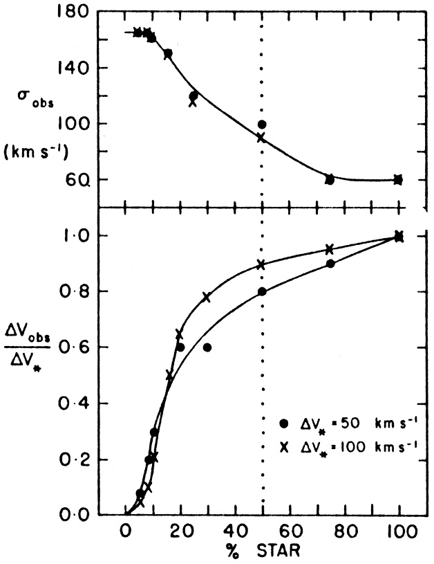Figure 32. Results of the Fourier quotient program for a mixture of two populations with different velocity dispersions. These experiments by McElroy (1981) model a composite spectrum by adding the spectrum of the nucleus of M31 ( = 165 km s-1) and that of a K0 III star broadened to a dispersion of * = 60 km s-1. The stellar component is shifted from the M31 spectrum by V* = 50 or 100 km s-1. Measured velocities and dispersions are shown by the points; the hand-drawn curves indicate the general trends. The upper panel shows that the measured dispersion is not a mean of 60 and 165 km s-1 weighted by the fractional light contribution of the star (abscissa) and galaxy. Rather, it is biased toward the smaller dispersion. This effect is much worse for the velocity Vobs: when the star contributes > 50% of the light, it dominates the velocity measurements almost completely.

More generally, there is little justification for the assumption that line profiles are everywhere Gaussian. Departures from Gaussians, even asymmetric profiles, may be common. For example, they may occur in ellipticals if the velocity ellipsoid becomes more and more radial at larger radii. These effects have not been studied, but they are likely to produce significant errors in V and (e.g., Simkin 1974).

Despite the above list of problems, Fourier quotient velocities and dispersions appear to be quite accurate when proper care is taken. Our confidence in the dispersion measures has been increased by the discovery (Terlevich et al. 1981, see section 4.2.4) that correlates with metallicity and that some discrepancies in average between different authors are due to different mean metallicities of the galaxies studied. Various Fourier techniques yield velocity dispersions which are internally consistent to ± 6% (Terlevich et al. 1981). However, there are still unexplained differences between Fourier and visual dispersion measurements.