


Having paid our mathematical dues, we are now prepared to examine the physics of gravitation as described by general relativity. This subject falls naturally into two pieces: how the curvature of spacetime acts on matter to manifest itself as "gravity", and how energy and momentum influence spacetime to create curvature. In either case it would be legitimate to start at the top, by stating outright the laws governing physics in curved spacetime and working out their consequences. Instead, we will try to be a little more motivational, starting with basic physical principles and attempting to argue that these lead naturally to an almost unique physical theory.
The most basic of these physical principles is the Principle of Equivalence, which comes in a variety of forms. The earliest form dates from Galileo and Newton, and is known as the Weak Equivalence Principle, or WEP. The WEP states that the "inertial mass" and "gravitational mass" of any object are equal. To see what this means, think about Newton's Second Law. This relates the force exerted on an object to the acceleration it undergoes, setting them proportional to each other with the constant of proportionality being the inertial mass mi:

| (4.1) |
The inertial mass clearly has a universal character, related to the
resistance you feel when you try to push on the object; it is the
same constant no matter what kind of force is being exerted. We also
have the law of gravitation, which states that the gravitational
force exerted on an object is proportional to the gradient of a scalar
field ![]() , known as the gravitational potential. The constant of
proportionality in this case is called the gravitational mass
mg:
, known as the gravitational potential. The constant of
proportionality in this case is called the gravitational mass
mg:

| (4.2) |
On the face of it, mg has a very different character than mi; it is a quantity specific to the gravitational force. If you like, it is the "gravitational charge" of the body. Nevertheless, Galileo long ago showed (apocryphally by dropping weights off of the Leaning Tower of Pisa, actually by rolling balls down inclined planes) that the response of matter to gravitation was universal - every object falls at the same rate in a gravitational field, independent of the composition of the object. In Newtonian mechanics this translates into the WEP, which is simply

| (4.3) |
for any object. An immediate consequence is that the behavior of freely-falling test particles is universal, independent of their mass (or any other qualities they may have); in fact we have

| (4.4) |
The universality of gravitation, as implied by the WEP, can be stated in another, more popular, form. Imagine that we consider a physicist in a tightly sealed box, unable to observe the outside world, who is doing experiments involving the motion of test particles, for example to measure the local gravitational field. Of course she would obtain different answers if the box were sitting on the moon or on Jupiter than she would on the Earth. But the answers would also be different if the box were accelerating at a constant velocity; this would change the acceleration of the freely-falling particles with respect to the box. The WEP implies that there is no way to disentangle the effects of a gravitational field from those of being in a uniformly accelerating frame, simply by observing the behavior of freely-falling particles. This follows from the universality of gravitation; it would be possible to distinguish between uniform acceleration and an electromagnetic field, by observing the behavior of particles with different charges. But with gravity it is impossible, since the "charge" is necessarily proportional to the (inertial) mass.
To be careful, we should limit our claims about the impossibility of distinguishing gravity from uniform acceleration by restricting our attention to "small enough regions of spacetime." If the sealed box were sufficiently big, the gravitational field would change from place to place in an observable way, while the effect of acceleration is always in the same direction. In a rocket ship or elevator, the particles always fall straight down:
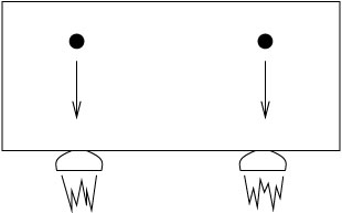
|
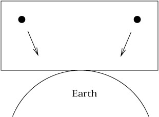
In a very big box in a gravitational field, however, the particles will move toward the center of the Earth (for example), which might be a different direction in different regions:
|
The WEP can therefore be stated as "the laws of freely-falling particles are the same in a gravitational field and a uniformly accelerated frame, in small enough regions of spacetime." In larger regions of spacetime there will be inhomogeneities in the gravitational field, which will lead to tidal forces which can be detected.
After the advent of special relativity, the concept of mass lost some of its uniqueness, as it became clear that mass was simply a manifestation of energy and momentum (E = mc2 and all that). It was therefore natural for Einstein to think about generalizing the WEP to something more inclusive. His idea was simply that there should be no way whatsoever for the physicist in the box to distinguish between uniform acceleration and an external gravitational field, no matter what experiments she did (not only by dropping test particles). This reasonable extrapolation became what is now known as the Einstein Equivalence Principle, or EEP: "In small enough regions of spacetime, the laws of physics reduce to those of special relativity; it is impossible to detect the existence of a gravitational field."
In fact, it is hard to imagine theories which respect the WEP but violate the EEP. Consider a hydrogen atom, a bound state of a proton and an electron. Its mass is actually less than the sum of the masses of the proton and electron considered individually, because there is a negative binding energy - you have to put energy into the atom to separate the proton and electron. According to the WEP, the gravitational mass of the hydrogen atom is therefore less than the sum of the masses of its constituents; the gravitational field couples to electromagnetism (which holds the atom together) in exactly the right way to make the gravitational mass come out right. This means that not only must gravity couple to rest mass universally, but to all forms of energy and momentum - which is practically the claim of the EEP. It is possible to come up with counterexamples, however; for example, we could imagine a theory of gravity in which freely falling particles began to rotate as they moved through a gravitational field. Then they could fall along the same paths as they would in an accelerated frame (thereby satisfying the WEP), but you could nevertheless detect the existence of the gravitational field (in violation of the EEP). Such theories seem contrived, but there is no law of nature which forbids them.
Sometimes a distinction is drawn between "gravitational laws of physics" and "non-gravitational laws of physics," and the EEP is defined to apply only to the latter. Then one defines the "Strong Equivalence Principle" (SEP) to include all of the laws of physics, gravitational and otherwise. I don't find this a particularly useful distinction, and won't belabor it. For our purposes, the EEP (or simply "the principle of equivalence") includes all of the laws of physics.
It is the EEP which implies (or at least suggests) that we should attribute the action of gravity to the curvature of spacetime. Remember that in special relativity a prominent role is played by inertial frames - while it was not possible to single out some frame of reference as uniquely "at rest", it was possible to single out a family of frames which were "unaccelerated" (inertial). The acceleration of a charged particle in an electromagnetic field was therefore uniquely defined with respect to these frames. The EEP, on the other hand, implies that gravity is inescapable - there is no such thing as a "gravitationally neutral object" with respect to which we can measure the acceleration due to gravity. It follows that "the acceleration due to gravity" is not something which can be reliably defined, and therefore is of little use.
Instead, it makes more sense to define "unaccelerated" as "freely falling," and that is what we shall do. This point of view is the origin of the idea that gravity is not a "force" - a force is something which leads to acceleration, and our definition of zero acceleration is "moving freely in the presence of whatever gravitational field happens to be around."
This seemingly innocuous step has profound implications for the nature of spacetime. In SR, we had a procedure for starting at some point and constructing an inertial frame which stretched throughout spacetime, by joining together rigid rods and attaching clocks to them. But, again due to inhomogeneities in the gravitational field, this is no longer possible. If we start in some freely-falling state and build a large structure out of rigid rods, at some distance away freely-falling objects will look like they are "accelerating" with respect to this reference frame, as shown in the figure on the next page.
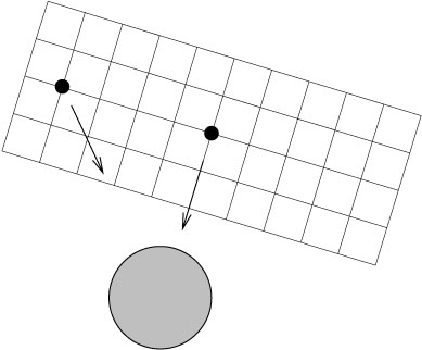
|
The solution is to retain the notion of inertial frames, but to discard the hope that they can be uniquely extended throughout space and time. Instead we can define locally inertial frames, those which follow the motion of freely falling particles in small enough regions of spacetime. (Every time we say "small enough regions", purists should imagine a limiting procedure in which we take the appropriate spacetime volume to zero.) This is the best we can do, but it forces us to give up a good deal. For example, we can no longer speak with confidence about the relative velocity of far away objects, since the inertial reference frames appropriate to those objects are independent of those appropriate to us.
So far we have been talking strictly about physics, without jumping to the conclusion that spacetime should be described as a curved manifold. It should be clear, however, why such a conclusion is appropriate. The idea that the laws of special relativity should be obeyed in sufficiently small regions of spacetime, and further that local inertial frames can be established in such regions, corresponds to our ability to construct Riemann normal coordinates at any one point on a manifold - coordinates in which the metric takes its canonical form and the Christoffel symbols vanish. The impossibility of comparing velocities (vectors) at widely separated regions corresponds to the path-dependence of parallel transport on a curved manifold. These considerations were enough to give Einstein the idea that gravity was a manifestation of spacetime curvature. But in fact we can be even more persuasive. (It is impossible to "prove" that gravity should be thought of as spacetime curvature, since scientific hypotheses can only be falsified, never verified [and not even really falsified, as Thomas Kuhn has famously argued]. But there is nothing to be dissatisfied with about convincing plausibility arguments, if they lead to empirically successful theories.)
Let's consider one of the celebrated predictions of the EEP, the
gravitational redshift. Consider two boxes, a distance z apart,
moving (far away from any matter, so we assume in the absence of any
gravitational field) with some constant acceleration a. At
time t0 the trailing box emits a photon of wavelength ![]() .
.

|
The boxes remain a constant distance apart, so the photon reaches
the leading box after a time
![]() t = z/c in the reference frame
of the boxes. In this time the boxes will have picked up an additional
velocity
t = z/c in the reference frame
of the boxes. In this time the boxes will have picked up an additional
velocity
![]() v = a
v = a![]() t = az/c. Therefore, the photon
reaching
the lead box will be redshifted by the conventional Doppler effect by
an amount
t = az/c. Therefore, the photon
reaching
the lead box will be redshifted by the conventional Doppler effect by
an amount
| (4.5) |
(We assume
![]() v/c is small, so we only work to first
order.)
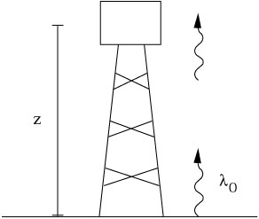
According to the EEP, the same thing should happen in a uniform
gravitational field. So we imagine a tower of height z sitting
on the surface of a planet, with ag the strength of
the gravitational
field (what Newton would have called the "acceleration due to gravity").
v/c is small, so we only work to first
order.)
According to the EEP, the same thing should happen in a uniform
gravitational field. So we imagine a tower of height z sitting
on the surface of a planet, with ag the strength of
the gravitational
field (what Newton would have called the "acceleration due to gravity").
|
This situation is supposed to be indistinguishable from the
previous one, from the point of view of an observer in a box at the top of
the tower (able to detect the emitted photon, but otherwise unable
to look outside the box). Therefore, a photon emitted from the
ground with wavelength ![]() should be redshifted by an amount
should be redshifted by an amount

| (4.6) |
This is the famous gravitational redshift. Notice that it is a
direct consequence of the EEP, not of the details of general
relativity. It has been verified experimentally, first by Pound
and Rebka in 1960. They used the Mössbauer effect to measure the
change in frequency in ![]() -rays as they traveled from the ground to
the top of Jefferson Labs at Harvard.
-rays as they traveled from the ground to
the top of Jefferson Labs at Harvard.
The formula for the redshift is more often stated in terms of the
Newtonian potential ![]() , where
, where
![]() =
= ![]()
![]() .
(The sign is changed with respect to the usual convention, since
we are thinking of
.
(The sign is changed with respect to the usual convention, since
we are thinking of ![]() as the acceleration of the reference
frame, not of a particle with respect to this reference frame.)
A non-constant gradient of
as the acceleration of the reference
frame, not of a particle with respect to this reference frame.)
A non-constant gradient of ![]() is like a time-varying
acceleration, and the equivalent net velocity is given by integrating
over the time between emission and absorption of the photon. We
then have
is like a time-varying
acceleration, and the equivalent net velocity is given by integrating
over the time between emission and absorption of the photon. We
then have
| (4.7) |
where
![]()
![]() is the total change in the gravitational potential,
and we have once again set c = 1. This simple formula for the
gravitational redshift continues to be true in more general
circumstances. Of course, by using the Newtonian potential at all,
we are restricting our domain of validity to weak gravitational
fields, but that is usually completely justified for observable
effects.
is the total change in the gravitational potential,
and we have once again set c = 1. This simple formula for the
gravitational redshift continues to be true in more general
circumstances. Of course, by using the Newtonian potential at all,
we are restricting our domain of validity to weak gravitational
fields, but that is usually completely justified for observable
effects.
The gravitational redshift leads to another argument that we should consider spacetime as curved. Consider the same experimental setup that we had before, now portrayed on the spacetime diagram on the next page.

|
The physicist on the ground emits a beam of light with wavelength
![]() from a height z0, which
travels to the top of the
tower at height z1. The time between when the
beginning of any
single wavelength of the light is emitted and the end of that same
wavelength is emitted is
from a height z0, which
travels to the top of the
tower at height z1. The time between when the
beginning of any
single wavelength of the light is emitted and the end of that same
wavelength is emitted is
![]() t0 =
t0 = ![]() /c, and the same time
interval for the absorption is
/c, and the same time
interval for the absorption is
![]() t1 =
t1 = ![]() /c. Since we imagine
that the gravitational field is not varying with time, the paths through
spacetime followed by the leading and trailing edge of the single
wave must be precisely congruent. (They are represented by some
generic curved paths, since we do not pretend that we know just what
the paths will be.) Simple geometry tells us that the times
/c. Since we imagine
that the gravitational field is not varying with time, the paths through
spacetime followed by the leading and trailing edge of the single
wave must be precisely congruent. (They are represented by some
generic curved paths, since we do not pretend that we know just what
the paths will be.) Simple geometry tells us that the times
![]() t0 and
t0 and
![]() t1 must be the same. But of course they
are not; the gravitational redshift implies that
t1 must be the same. But of course they
are not; the gravitational redshift implies that
![]() t1 >
t1 > ![]() t0. (Which we can interpret as "the
clock on the tower
appears to run more quickly.") The fault lies with "simple
geometry"; a better description of what happens is to imagine that
spacetime is curved.
t0. (Which we can interpret as "the
clock on the tower
appears to run more quickly.") The fault lies with "simple
geometry"; a better description of what happens is to imagine that
spacetime is curved.
All of this should constitute more than enough motivation for our
claim that, in the presence of gravity, spacetime should be thought
of as a curved manifold. Let us now take this to be true and begin
to set up how physics works in a curved spacetime. The principle
of equivalence tells us that the laws of physics, in small enough
regions of spacetime, look like those of special relativity. We
interpret this in the language of manifolds as the statement that
these laws, when written in Riemannian normal coordinates x![]() based at some point p, are described by equations which take the
same form as they would in flat space. The simplest example is
that of freely-falling (unaccelerated) particles. In flat space
such particles move in straight lines; in equations, this is
expressed as the vanishing of the second derivative of the parameterized
path
x
based at some point p, are described by equations which take the
same form as they would in flat space. The simplest example is
that of freely-falling (unaccelerated) particles. In flat space
such particles move in straight lines; in equations, this is
expressed as the vanishing of the second derivative of the parameterized
path
x![]() (
(![]() ):
):

| (4.8) |
According to the EEP, exactly this equation should hold in
curved space, as long as the coordinates x![]() are RNC's. What
about some other coordinate system? As it stands, (4.8) is
not an equation between tensors. However, there is a unique
tensorial equation which reduces to (4.8) when the Christoffel
symbols vanish; it is
are RNC's. What
about some other coordinate system? As it stands, (4.8) is
not an equation between tensors. However, there is a unique
tensorial equation which reduces to (4.8) when the Christoffel
symbols vanish; it is
| (4.9) |
Of course, this is simply the geodesic equation. In general relativity, therefore, free particles move along geodesics; we have mentioned this before, but now you know why it is true.
As far as free particles go, we have argued that curvature of
spacetime is necessary to describe gravity; we have not yet shown that
it is sufficient. To do so, we can show how the usual results of
Newtonian gravity fit into the picture. We define the "Newtonian
limit" by three requirements: the particles are moving slowly
(with respect to the speed of light), the gravitational field is
weak (can be considered a perturbation of flat space), and the field
is also static (unchanging with time). Let us see what these
assumptions do to the geodesic equation, taking the proper time
![]() as an affine parameter. "Moving slowly" means that
as an affine parameter. "Moving slowly" means that

| (4.10) |
so the geodesic equation becomes
| (4.11) |
Since the field is static, the relevant Christoffel symbols
![]() simplify:
simplify:
| (4.12) |
Finally, the weakness of the gravitational field allows us to decompose the metric into the Minkowski form plus a small perturbation:
| (4.13) |
(We are working in Cartesian coordinates, so
![]() is the
canonical form of the metric. The "smallness condition" on
the metric perturbation
h
is the
canonical form of the metric. The "smallness condition" on
the metric perturbation
h![]()
![]() doesn't really make sense in
other coordinates.) From the definition of the inverse metric,
g
doesn't really make sense in
other coordinates.) From the definition of the inverse metric,
g![]()
![]() g
g![]()
![]() =
= ![]() , we find that to first
order in h,
, we find that to first
order in h,
| (4.14) |
where
h![]()
![]() =
= ![]()
![]() h
h![]()
![]() . In
fact, we can use the Minkowski metric to raise and lower indices on
an object of any definite order in h, since the corrections would
only contribute at higher orders.
. In
fact, we can use the Minkowski metric to raise and lower indices on
an object of any definite order in h, since the corrections would
only contribute at higher orders.
Putting it all together, we find
| (4.15) |
The geodesic equation (4.11) is therefore
| (4.16) |
Using
![]() h00 = 0, the
h00 = 0, the ![]() = 0 component of this is just
= 0 component of this is just

| (4.17) |
That is,
![]() is constant. To examine the spacelike
components of (4.16), recall that the spacelike components of
is constant. To examine the spacelike
components of (4.16), recall that the spacelike components of
![]() are just those of a 3 × 3 identity
matrix. We therefore have
are just those of a 3 × 3 identity
matrix. We therefore have
| (4.18) |
Dividing both sides by
![]()
![]()
![]() has the
effect of converting the derivative on the left-hand side
from
has the
effect of converting the derivative on the left-hand side
from ![]() to t, leaving us with
to t, leaving us with

| (4.19) |
This begins to look a great deal like Newton's theory of gravitation. In fact, if we compare this equation to (4.4), we find that they are the same once we identify

| (4.20) |
or in other words
| (4.21) |
Therefore, we have shown that the curvature of spacetime is indeed sufficient to describe gravity in the Newtonian limit, as long as the metric takes the form (4.21). It remains, of course, to find field equations for the metric which imply that this is the form taken, and that for a single gravitating body we recover the Newtonian formula

| (4.22) |
but that will come soon enough.
Our next task is to show how the remaining laws of physics, beyond those governing freely-falling particles, adapt to the curvature of spacetime. The procedure essentially follows the paradigm established in arguing that free particles move along geodesics. Take a law of physics in flat space, traditionally written in terms of partial derivatives and the flat metric. According to the equivalence principle this law will hold in the presence of gravity, as long as we are in Riemannian normal coordinates. Translate the law into a relationship between tensors; for example, change partial derivatives to covariant ones. In RNC's this version of the law will reduce to the flat-space one, but tensors are coordinate-independent objects, so the tensorial version must hold in any coordinate system.
This procedure is sometimes given a name, the Principle of Covariance. I'm not sure that it deserves its own name, since it's really a consequence of the EEP plus the requirement that the laws of physics be independent of coordinates. (The requirement that laws of physics be independent of coordinates is essentially impossible to even imagine being untrue. Given some experiment, if one person uses one coordinate system to predict a result and another one uses a different coordinate system, they had better agree.) Another name is the "comma-goes-to-semicolon rule", since at a typographical level the thing you have to do is replace partial derivatives (commas) with covariant ones (semicolons).
We have already implicitly used the principle of covariance (or
whatever you want to call it) in deriving the statement that free
particles move along geodesics. For the most part, it is very simple
to apply it to interesting cases. Consider for example the formula
for conservation of energy in flat spacetime,
![]() T
T![]()
![]() = 0.
The adaptation to curved spacetime is immediate:
= 0.
The adaptation to curved spacetime is immediate:

| (4.23) |
This equation expresses the conservation of energy in the presence of a gravitational field.
Unfortunately, life is not always so easy. Consider Maxwell's
equations in special relativity, where it would seem that the principle
of covariance can be applied in a straightforward way. The
inhomogeneous equation
![]() F
F![]()
![]() = 4
= 4![]() J
J![]() becomes
becomes
| (4.24) |
and the homogeneous one
![]() F
F![]()
![]() ] = 0 becomes
] = 0 becomes

| (4.25) |
On the other hand, we could also write Maxwell's equations in flat space in terms of differential forms as
| (4.26) |
and

| (4.27) |
These are already in perfectly tensorial form, since we have shown
that the exterior derivative is a well-defined tensor operator regardless
of what the connection is. We therefore begin to worry a little bit;
what is the guarantee that the process of writing a law of physics in
tensorial form gives a unique answer? In fact, as we have mentioned
earlier, the differential forms versions of Maxwell's equations should
be taken as fundamental. Nevertheless, in this case it happens to make no
difference, since in the absence of torsion (4.26) is identical to (4.24),
and (4.27) is identical to (4.25); the symmetric part of the connection
doesn't contribute. Similarly, the definition of the field strength tensor
in terms of the potential A![]() can be written either as
can be written either as
| (4.28) |
or equally well as

| (4.29) |
The worry about uniqueness is a real one, however. Imagine that
two vector fields X![]() and Y
and Y![]() obey a law in flat space
given by
obey a law in flat space
given by
| (4.30) |
The problem in writing this as a tensor equation should be clear: the partial derivatives can be commuted, but covariant derivatives cannot. If we simply replace the partials in (4.30) by covariant derivatives, we get a different answer than we would if we had first exchanged the order of the derivatives (leaving the equation in flat space invariant) and then replaced them. The difference is given by

| (4.31) |
The prescription for generalizing laws from flat to curved spacetimes does not guide us in choosing the order of the derivatives, and therefore is ambiguous about whether a term such as that in (4.31) should appear in the presence of gravity. (The problem of ordering covariant derivatives is similar to the problem of operator-ordering ambiguities in quantum mechanics.)
In the literature you can find various prescriptions for dealing with ambiguities such as this, most of which are sensible pieces of advice such as remembering to preserve gauge invariance for electromagnetism. But deep down the real answer is that there is no way to resolve these problems by pure thought alone; the fact is that there may be more than one way to adapt a law of physics to curved space, and ultimately only experiment can decide between the alternatives.
In fact, let us be honest about the principle of equivalence: it serves as a useful guideline, but it does not deserve to be treated as a fundamental principle of nature. From the modern point of view, we do not expect the EEP to be rigorously true. Consider the following alternative version of (4.24):
| (4.32) |
where R is the Ricci scalar and ![]() is some coupling constant.
If this equation correctly described electrodynamics in curved
spacetime, it would be possible to measure R even in an arbitrarily
small region, by doing experiments with charged particles. The
equivalence principle therefore demands that
is some coupling constant.
If this equation correctly described electrodynamics in curved
spacetime, it would be possible to measure R even in an arbitrarily
small region, by doing experiments with charged particles. The
equivalence principle therefore demands that ![]() = 0. But
otherwise this is a perfectly respectable equation, consistent with
charge conservation and other desirable features of electromagnetism,
which reduces to the usual equation in flat space. Indeed, in a
world governed by quantum mechanics we expect all possible couplings
between different fields (such as gravity and electromagnetism) that
are consistent with the symmetries of the theory (in this case,
gauge invariance). So why is it reasonable to set
= 0. But
otherwise this is a perfectly respectable equation, consistent with
charge conservation and other desirable features of electromagnetism,
which reduces to the usual equation in flat space. Indeed, in a
world governed by quantum mechanics we expect all possible couplings
between different fields (such as gravity and electromagnetism) that
are consistent with the symmetries of the theory (in this case,
gauge invariance). So why is it reasonable to set ![]() = 0? The
real reason is one of scales. Notice that the Ricci tensor involves
second derivatives of the metric, which is dimensionless, so R
has dimensions of (length)-2 (with c = 1). Therefore
= 0? The
real reason is one of scales. Notice that the Ricci tensor involves
second derivatives of the metric, which is dimensionless, so R
has dimensions of (length)-2 (with c = 1). Therefore ![]() must
have dimensions of (length)2. But since the coupling
represented by
must
have dimensions of (length)2. But since the coupling
represented by
![]() is of gravitational origin, the only reasonable
expectation for the relevant length scale is
is of gravitational origin, the only reasonable
expectation for the relevant length scale is

| (4.33) |
where lP is the Planck length
| (4.34) |
where ![]() is of course Planck's constant. So the length scale
corresponding to this coupling is extremely small, and for any
conceivable experiment we expect the typical scale of variation for
the gravitational field to be much larger. Therefore the reason why
this equivalence-principle-violating term can be safely ignored is
simply because
is of course Planck's constant. So the length scale
corresponding to this coupling is extremely small, and for any
conceivable experiment we expect the typical scale of variation for
the gravitational field to be much larger. Therefore the reason why
this equivalence-principle-violating term can be safely ignored is
simply because ![]() R is probably a fantastically small number, far
out of the reach of any experiment. On the other hand, we might as
well keep an open mind, since our expectations are not always borne
out by observation.
R is probably a fantastically small number, far
out of the reach of any experiment. On the other hand, we might as
well keep an open mind, since our expectations are not always borne
out by observation.
Having established how physical laws govern the behavior of fields and objects in a curved spacetime, we can complete the establishment of general relativity proper by introducing Einstein's field equations, which govern how the metric responds to energy and momentum. We will actually do this in two ways: first by an informal argument close to what Einstein himself was thinking, and then by starting with an action and deriving the corresponding equations of motion.
The informal argument begins with the realization that we would like to find an equation which supersedes the Poisson equation for the Newtonian potential:

| (4.35) |
where
![]() =
= ![]()
![]()
![]() is the Laplacian in
space and
is the Laplacian in
space and ![]() is the mass density. (The explicit form of
is the mass density. (The explicit form of
![]() given in (4.22) is one solution of (4.35),
for the case of a pointlike mass distribution.) What characteristics
should our sought-after equation possess? On the left-hand side
of (4.35) we have a second-order differential operator acting on the
gravitational potential, and on the right-hand side a measure of
the mass distribution. A relativistic generalization should take
the form of an equation between tensors. We know what the tensor
generalization of the mass density is; it's the energy-momentum
tensor
T
given in (4.22) is one solution of (4.35),
for the case of a pointlike mass distribution.) What characteristics
should our sought-after equation possess? On the left-hand side
of (4.35) we have a second-order differential operator acting on the
gravitational potential, and on the right-hand side a measure of
the mass distribution. A relativistic generalization should take
the form of an equation between tensors. We know what the tensor
generalization of the mass density is; it's the energy-momentum
tensor
T![]()
![]() . The gravitational potential,
meanwhile, should
get replaced by the metric tensor. We might therefore guess
that our new equation will have
T
. The gravitational potential,
meanwhile, should
get replaced by the metric tensor. We might therefore guess
that our new equation will have
T![]()
![]() set proportional to some
tensor which is second-order in derivatives of the metric. In
fact, using (4.21) for the metric in the Newtonian limit and
T00 =
set proportional to some
tensor which is second-order in derivatives of the metric. In
fact, using (4.21) for the metric in the Newtonian limit and
T00 = ![]() , we see that in this limit we are looking for an
equation that predicts
, we see that in this limit we are looking for an
equation that predicts
| (4.36) |
but of course we want it to be completely tensorial.
The left-hand side of (4.36) does not obviously generalize to
a tensor. The first choice might be to act the D'Alembertian
![]() =
= ![]()
![]() on the metric
g
on the metric
g![]()
![]() , but this
is automatically zero by metric compatibility. Fortunately, there
is an obvious quantity which is not zero and is constructed from
second derivatives (and first derivatives) of the metric: the
Riemann tensor
R
, but this
is automatically zero by metric compatibility. Fortunately, there
is an obvious quantity which is not zero and is constructed from
second derivatives (and first derivatives) of the metric: the
Riemann tensor
R![]()
![]()
![]()
![]() . It doesn't have the right
number of indices, but we can contract it to form the Ricci tensor
R
. It doesn't have the right
number of indices, but we can contract it to form the Ricci tensor
R![]()
![]() , which does (and is symmetric to
boot). It is therefore
reasonable to guess that the gravitational field equations are
, which does (and is symmetric to
boot). It is therefore
reasonable to guess that the gravitational field equations are

| (4.37) |
for some constant ![]() . In fact, Einstein did suggest this
equation at one point. There is a problem, unfortunately, with
conservation of energy. According to the Principle of Equivalence,
the statement of energy-momentum conservation in curved spacetime
should be
. In fact, Einstein did suggest this
equation at one point. There is a problem, unfortunately, with
conservation of energy. According to the Principle of Equivalence,
the statement of energy-momentum conservation in curved spacetime
should be

| (4.38) |
which would then imply

| (4.39) |
This is certainly not true in an arbitrary geometry; we have seen from the Bianchi identity (3.94) that
| (4.40) |
But our proposed field equation implies that
R = ![]() g
g![]()
![]() T
T![]()
![]() =
= ![]() T, so taking these together we have
T, so taking these together we have

| (4.41) |
The covariant derivative of a scalar is just the partial derivative, so (4.41) is telling us that T is constant throughout spacetime. This is highly implausible, since T = 0 in vacuum while T > 0 in matter. We have to try harder.
(Actually we are cheating slightly, in taking the equation
![]() T
T![]()
![]() = 0 so seriously. If as we said, the
equivalence
principle is only an approximate guide, we could imagine that there are
nonzero terms on the right-hand side involving the curvature tensor.
Later we will be more precise and argue that they are strictly zero.)
= 0 so seriously. If as we said, the
equivalence
principle is only an approximate guide, we could imagine that there are
nonzero terms on the right-hand side involving the curvature tensor.
Later we will be more precise and argue that they are strictly zero.)
Of course we don't have to try much harder, since we already know of a symmetric (0, 2) tensor, constructed from the Ricci tensor, which is automatically conserved: the Einstein tensor
| (4.42) |
which always obeys
![]() G
G![]()
![]() = 0. We are therefore led to
propose
= 0. We are therefore led to
propose

| (4.43) |
as a field equation for the metric. This equation satisfies all of the obvious requirements; the right-hand side is a covariant expression of the energy and momentum density in the form of a symmetric and conserved (0, 2) tensor, while the left-hand side is a symmetric and conserved (0, 2) tensor constructed from the metric and its first and second derivatives. It only remains to see whether it actually reproduces gravity as we know it.
To answer this, note that contracting both sides of (4.43) yields (in four dimensions)

| (4.44) |
and using this we can rewrite (4.43) as
| (4.45) |
This is the same equation, just written slightly differently. We would
like to see if it predicts Newtonian gravity in the weak-field,
time-independent, slowly-moving-particles limit. In this limit the
rest energy
![]() = T00 will be much larger than the
other terms in
T
= T00 will be much larger than the
other terms in
T![]()
![]() , so we want to focus on the
, so we want to focus on the ![]() = 0,
= 0, ![]() = 0
component of (4.45). In the weak-field limit, we write (in accordance
with (4.13) and (4.14))
= 0
component of (4.45). In the weak-field limit, we write (in accordance
with (4.13) and (4.14))
| (4.46) |
The trace of the energy-momentum tensor, to lowest nontrivial order, is
| (4.47) |
Plugging this into (4.45), we get

| (4.48) |
This is an equation relating derivatives of the metric to the
energy density. To find the explicit expression in terms of the
metric, we need to evaluate
R00 = R![]() 0
0![]() 0.
In fact we only need
Ri0i0, since
R0000 = 0. We have
0.
In fact we only need
Ri0i0, since
R0000 = 0. We have

| (4.49) |
The second term here is a time derivative, which vanishes for
static fields. The third and fourth terms are of the form
(![]() )2,
and since
)2,
and since ![]() is first-order in the metric perturbation these
contribute only at second order, and can be neglected. We are left
with
Ri0j0 =
is first-order in the metric perturbation these
contribute only at second order, and can be neglected. We are left
with
Ri0j0 = ![]()
![]() . From this we get
. From this we get
| (4.50) |
Comparing to (4.48), we see that the 00 component of (4.43) in the Newtonian limit predicts
| (4.51) |
But this is exactly (4.36), if we set
![]() = 8
= 8![]() G.
G.
So our guess seems to have worked out. With the normalization fixed by comparison with the Newtonian limit, we can present Einstein's equations for general relativity:
| (4.52) |
These tell us how the curvature of spacetime reacts to the presence of energy-momentum. Einstein, you may have heard, thought that the left-hand side was nice and geometrical, while the right-hand side was somewhat less compelling.
Einstein's equations may be thought of as second-order differential
equations for the metric tensor field g![]()
![]() . There are ten
independent equations (since both sides are symmetric two-index
tensors), which seems to be exactly right for the ten unknown functions
of the metric components. However, the Bianchi identity
. There are ten
independent equations (since both sides are symmetric two-index
tensors), which seems to be exactly right for the ten unknown functions
of the metric components. However, the Bianchi identity
![]() G
G![]()
![]() = 0 represents four constraints on the
functions
R
= 0 represents four constraints on the
functions
R![]()
![]() , so
there are only six truly independent equations in (4.52). In fact
this is appropriate, since if a metric is a solution to Einstein's
equation in one coordinate system x
, so
there are only six truly independent equations in (4.52). In fact
this is appropriate, since if a metric is a solution to Einstein's
equation in one coordinate system x![]() it should also be a
solution in any other coordinate system x
it should also be a
solution in any other coordinate system x![]() . This means that
there are four unphysical degrees of freedom in
g
. This means that
there are four unphysical degrees of freedom in
g![]()
![]() (represented
by the four functions
x
(represented
by the four functions
x![]() (x
(x![]() )), and we should expect that
Einstein's equations only constrain the six coordinate-independent
degrees of freedom.
)), and we should expect that
Einstein's equations only constrain the six coordinate-independent
degrees of freedom.
As differential equations, these are
extremely complicated; the Ricci scalar and tensor are contractions
of the Riemann tensor, which involves derivatives and products
of the Christoffel symbols, which in turn involve the inverse metric
and derivatives of the metric. Furthermore, the energy-momentum
tensor
T![]()
![]() will generally involve the metric as
well. The
equations are also nonlinear, so that two known solutions cannot
be superposed to find a third. It is therefore very difficult to
solve Einstein's equations in any sort of generality, and it is
usually necessary to make some simplifying assumptions. Even
in vacuum, where we set the energy-momentum tensor to zero, the
resulting equations (from (4.45))
will generally involve the metric as
well. The
equations are also nonlinear, so that two known solutions cannot
be superposed to find a third. It is therefore very difficult to
solve Einstein's equations in any sort of generality, and it is
usually necessary to make some simplifying assumptions. Even
in vacuum, where we set the energy-momentum tensor to zero, the
resulting equations (from (4.45))

| (4.53) |
can be very difficult to solve. The most popular sort of simplifying assumption is that the metric has a significant degree of symmetry, and we will talk later on about how symmetries of the metric make life easier.
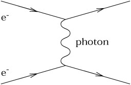
The nonlinearity of general relativity is worth remarking on. In Newtonian gravity the potential due to two point masses is simply the sum of the potentials for each mass, but clearly this does not carry over to general relativity (outside the weak-field limit). There is a physical reason for this, namely that in GR the gravitational field couples to itself. This can be thought of as a consequence of the equivalence principle - if gravitation did not couple to itself, a "gravitational atom" (two particles bound by their mutual gravitational attraction) would have a different inertial mass (due to the negative binding energy) than gravitational mass. From a particle physics point of view this can be expressed in terms of Feynman diagrams. The electromagnetic interaction between two electrons can be thought of as due to exchange of a virtual photon:
|
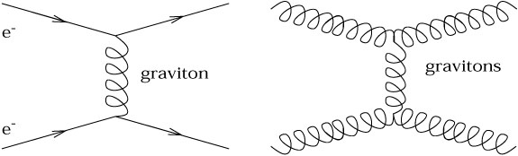
But there is no diagram in which two photons exchange another photon between themselves; electromagnetism is linear. The gravitational interaction, meanwhile, can be thought of as due to exchange of a virtual graviton (a quantized perturbation of the metric). The nonlinearity manifests itself as the fact that both electrons and gravitons (and anything else) can exchange virtual gravitons, and therefore exert a gravitational force:
|
There is nothing profound about this feature of gravity; it is shared by most gauge theories, such as quantum chromodynamics, the theory of the strong interactions. (Electromagnetism is actually the exception; the linearity can be traced to the fact that the relevant gauge group, U(1), is abelian.) But it does represent a departure from the Newtonian theory. (Of course this quantum mechanical language of Feynman diagrams is somewhat inappropriate for GR, which has not [yet] been successfully quantized, but the diagrams are just a convenient shorthand for remembering what interactions exist in the theory.)
To increase your confidence that Einstein's equations as we have derived them are indeed the correct field equations for the metric, let's see how they can be derived from a more modern viewpoint, starting from an action principle. (In fact the equations were first derived by Hilbert, not Einstein, and Hilbert did it using the action principle. But he had been inspired by Einstein's previous papers on the subject, and Einstein himself derived the equations independently, so they are rightly named after Einstein. The action, however, is rightly called the Hilbert action.) The action should be the integral over spacetime of a Lagrange density ("Lagrangian" for short, although strictly speaking the Lagrangian is the integral over space of the Lagrange density):
| (4.54) |
The Lagrange density is a tensor density, which can be written as
![]() times a scalar. What scalars can we make out of the
metric?
Since we know that the metric can be set equal to its canonical form
and its first derivatives set to zero at any one point, any nontrivial
scalar must involve at least second derivatives of the metric.
The Riemann tensor is of course made from second derivatives of the
metric, and we argued earlier that the only independent scalar we
could construct from the Riemann tensor was the Ricci scalar
R. What we did not show, but is nevertheless true, is that any
nontrivial tensor made from the metric and its first and second
derivatives can be expressed in terms of the metric and the Riemann
tensor. Therefore, the only independent scalar constructed from
the metric, which is no higher than second order in its derivatives,
is the Ricci scalar. Hilbert figured that this was therefore the
simplest possible choice for a Lagrangian, and proposed
times a scalar. What scalars can we make out of the
metric?
Since we know that the metric can be set equal to its canonical form
and its first derivatives set to zero at any one point, any nontrivial
scalar must involve at least second derivatives of the metric.
The Riemann tensor is of course made from second derivatives of the
metric, and we argued earlier that the only independent scalar we
could construct from the Riemann tensor was the Ricci scalar
R. What we did not show, but is nevertheless true, is that any
nontrivial tensor made from the metric and its first and second
derivatives can be expressed in terms of the metric and the Riemann
tensor. Therefore, the only independent scalar constructed from
the metric, which is no higher than second order in its derivatives,
is the Ricci scalar. Hilbert figured that this was therefore the
simplest possible choice for a Lagrangian, and proposed

| (4.55) |
The equations of motion should come from varying the action
with respect to the metric. In fact let us consider variations
with respect to the inverse metric
g![]()
![]() , which are slightly
easier but give an equivalent set of equations. Using
R = g
, which are slightly
easier but give an equivalent set of equations. Using
R = g![]()
![]() R
R![]()
![]() , in general we will have
, in general we will have
| (4.56) |
The second term
(![]() S)2 is already in the form of some
expression times
S)2 is already in the form of some
expression times
![]() g
g![]()
![]() ; let's examine the others more
closely.
; let's examine the others more
closely.
Recall that the Ricci tensor is the contraction of the Riemann tensor, which is given by
| (4.57) |
The variation of this with respect the metric can be found first varying the connection with respect to the metric, and then substituting into this expression. Let us however consider arbitrary variations of the connection, by replacing
| (4.58) |
The variation
![]()
![]() is the difference of
two connections, and therefore is itself a tensor. We can thus
take its covariant derivative,
is the difference of
two connections, and therefore is itself a tensor. We can thus
take its covariant derivative,

| (4.59) |
Given this expression (and a small amount of labor) it is easy to show that
| (4.60) |
You can check this yourself. Therefore, the contribution of
the first term in (4.56) to ![]() S can be written
S can be written
| (4.61) |
where we have used metric compatibility and relabeled some dummy indices. But now we have the integral with respect to the natural volume element of the covariant divergence of a vector; by Stokes's theorem, this is equal to a boundary contribution at infinity which we can set to zero by making the variation vanish at infinity. (We haven't actually shown that Stokes's theorem, as mentioned earlier in terms of differential forms, can be thought of this way, but you can easily convince yourself it's true.) Therefore this term contributes nothing to the total variation.
To make sense of the
(![]() S)3 term we need to use the following
fact, true for any matrix M:
S)3 term we need to use the following
fact, true for any matrix M:
| (4.62) |
Here, ln M is defined by exp(ln M) = M. (For numbers this is obvious, for matrices it's a little less straightforward.) The variation of this identity yields
| (4.63) |
Here we have used the cyclic property of the trace to allow us to
ignore the fact that M-1 and ![]() M may not commute. Now we
would like to apply this to the inverse metric,
M = g
M may not commute. Now we
would like to apply this to the inverse metric,
M = g![]()
![]() . Then
detM = g-1 (where
g = detg
. Then
detM = g-1 (where
g = detg![]()
![]() ), and
), and
| (4.64) |
Now we can just plug in:
| (4.65) |
Hearkening back to (4.56), and remembering that
(![]() S)1 does
not contribute, we find
S)1 does
not contribute, we find
| (4.66) |
This should vanish for arbitrary variations, so we are led to Einstein's equations in vacuum:
| (4.67) |
The fact that this simple action leads to the same vacuum field equations as we had previously arrived at by more informal arguments certainly reassures us that we are doing something right. What we would really like, however, is to get the non-vacuum field equations as well. That means we consider an action of the form
| (4.68) |
where SM is the action for matter, and we have presciently normalized the gravitational action (although the proper normalization is somewhat convention-dependent). Following through the same procedure as above leads to
| (4.69) |
and we recover Einstein's equations if we can set
| (4.70) |
What makes us think that we can make such an identification? In fact (4.70) turns out to be the best way to define a symmetric energy-momentum tensor. The tricky part is to show that it is conserved, which is in fact automatically true, but which we will not justify until the next section.
We say that (4.70) provides the "best" definition of the energy-momentum
tensor because it is not the only one you will find. In flat Minkowski
space, there is an alternative definition which is sometimes given in books
on electromagnetism or field theory. In this context energy-momentum
conservation arises as a consequence of symmetry of the Lagrangian
under spacetime translations. Noether's theorem
states that every symmetry of a Lagrangian implies the existence
of a conservation law; invariance under the four spacetime translations
leads to a tensor
S![]()
![]() which obeys
which obeys
![]() S
S![]()
![]() = 0 (four relations,
one for each value of
= 0 (four relations,
one for each value of ![]() ). The details can be found in Wald or
in any number of field theory books. Applying Noether's procedure
to a Lagrangian which depends on some fields
). The details can be found in Wald or
in any number of field theory books. Applying Noether's procedure
to a Lagrangian which depends on some fields ![]() and their
first derivatives
and their
first derivatives
![]()
![]() , we obtain
, we obtain
| (4.71) |
where a sum over i is implied. You can check that this tensor
is conserved by virtue of the equations of motion of the matter
fields.
S![]()
![]() often goes by the name "canonical
energy-momentum tensor"; however, there are a number of reasons
why it is more convenient for us to use (4.70). First and foremost,
(4.70) is in fact what appears on the right hand side of
Einstein's equations when they are derived from an action, and it
is not always possible to generalize (4.71) to curved spacetime.
But even in flat space (4.70) has its advantages; it is
manifestly symmetric, and also guaranteed to be gauge invariant,
neither of which is true for (4.71). We will therefore stick with
(4.70) as the definition of the energy-momentum tensor.
often goes by the name "canonical
energy-momentum tensor"; however, there are a number of reasons
why it is more convenient for us to use (4.70). First and foremost,
(4.70) is in fact what appears on the right hand side of
Einstein's equations when they are derived from an action, and it
is not always possible to generalize (4.71) to curved spacetime.
But even in flat space (4.70) has its advantages; it is
manifestly symmetric, and also guaranteed to be gauge invariant,
neither of which is true for (4.71). We will therefore stick with
(4.70) as the definition of the energy-momentum tensor.
Sometimes it is useful to think about Einstein's equations without
specifying the theory of matter from which
T![]()
![]() is derived.
This leaves us with a great deal of arbitrariness; consider for
example the question "What metrics obey Einstein's equations?"
In the absence of some constraints on
T
is derived.
This leaves us with a great deal of arbitrariness; consider for
example the question "What metrics obey Einstein's equations?"
In the absence of some constraints on
T![]()
![]() , the answer is "any
metric at all"; simply take the metric of your choice, compute the
Einstein tensor
G
, the answer is "any
metric at all"; simply take the metric of your choice, compute the
Einstein tensor
G![]()
![]() for this metric, and then demand that
T
for this metric, and then demand that
T![]()
![]() be equal to
G
be equal to
G![]()
![]() . (It will automatically be conserved,
by the Bianchi identity.) Our real concern is with the existence
of solutions to Einstein's equations in the presence of "realistic"
sources of energy and momentum, whatever that means. The most
common property that is demanded of
T
. (It will automatically be conserved,
by the Bianchi identity.) Our real concern is with the existence
of solutions to Einstein's equations in the presence of "realistic"
sources of energy and momentum, whatever that means. The most
common property that is demanded of
T![]()
![]() is that it represent
positive energy densities - no negative masses are allowed. In
a locally inertial frame this requirement can be stated as
is that it represent
positive energy densities - no negative masses are allowed. In
a locally inertial frame this requirement can be stated as
![]() = T00
= T00 ![]() 0. To turn this into a coordinate-independent
statement, we ask that
0. To turn this into a coordinate-independent
statement, we ask that

| (4.72) |
This is known as the Weak Energy Condition, or WEC. It seems like a fairly reasonable requirement, and many of the important theorems about solutions to general relativity (such as the singularity theorems of Hawking and Penrose) rely on this condition or something very close to it. Unfortunately it is not set in stone; indeed, it is straightforward to invent otherwise respectable classical field theories which violate the WEC, and almost impossible to invent a quantum field theory which obeys it. Nevertheless, it is legitimate to assume that the WEC holds in all but the most extreme conditions. (There are also stronger energy conditions, but they are even less true than the WEC, and we won't dwell on them.)
We have now justified Einstein's equations in two different ways: as the natural covariant generalization of Poisson's equation for the Newtonian gravitational potential, and as the result of varying the simplest possible action we could invent for the metric. The rest of the course will be an exploration of the consequences of these equations, but before we start on that road let us briefly explore ways in which the equations could be modified. There are an uncountable number of such ways, but we will consider four different possibilities: the introduction of a cosmological constant, higher-order terms in the action, gravitational scalar fields, and a nonvanishing torsion tensor.
The first possibility is the cosmological constant; George Gamow has quoted Einstein as calling this the biggest mistake of his life. Recall that in our search for the simplest possible action for gravity we noted that any nontrivial scalar had to be of at least second order in derivatives of the metric; at lower order all we can create is a constant. Although a constant does not by itself lead to very interesting dynamics, it has an important effect if we add it to the conventional Hilbert action. We therefore consider an action given by
| (4.73) |
where ![]() is some constant. The resulting field equations
are
is some constant. The resulting field equations
are
| (4.74) |
and of course there would be an energy-momentum tensor on the
right hand side if we had included an action for matter. ![]() is the cosmological constant; it was originally introduced by
Einstein after it became clear that there were no solutions to his
equations representing a static cosmology (a universe unchanging
with time on large scales) with a nonzero matter content. If the
cosmological constant is tuned just right, it is possible to find
a static solution, but it is unstable to small perturbations.
Furthermore, once Hubble demonstrated that the universe is expanding,
it became less important to find static solutions, and Einstein
rejected his suggestion. Like Rasputin, however, the cosmological
constant has proven difficult to kill off. If we like we can move
the additional term in (4.74) to the right hand side, and think
of it as a kind of energy-momentum tensor, with
T
is the cosmological constant; it was originally introduced by
Einstein after it became clear that there were no solutions to his
equations representing a static cosmology (a universe unchanging
with time on large scales) with a nonzero matter content. If the
cosmological constant is tuned just right, it is possible to find
a static solution, but it is unstable to small perturbations.
Furthermore, once Hubble demonstrated that the universe is expanding,
it became less important to find static solutions, and Einstein
rejected his suggestion. Like Rasputin, however, the cosmological
constant has proven difficult to kill off. If we like we can move
the additional term in (4.74) to the right hand side, and think
of it as a kind of energy-momentum tensor, with
T![]()
![]() = -
= - ![]() g
g![]()
![]() (it is automatically conserved by
metric compatibility).
Then
(it is automatically conserved by
metric compatibility).
Then ![]() can be interpreted as the "energy density of the
vacuum," a source of energy and momentum that is present even in
the absence of matter fields. This interpretation is important because
quantum field theory predicts that the vacuum should have some sort
of energy and momentum. In ordinary quantum mechanics, an harmonic
oscillator with frequency
can be interpreted as the "energy density of the
vacuum," a source of energy and momentum that is present even in
the absence of matter fields. This interpretation is important because
quantum field theory predicts that the vacuum should have some sort
of energy and momentum. In ordinary quantum mechanics, an harmonic
oscillator with frequency ![]() and minimum classical energy
E0 = 0 upon quantization has a ground state with energy
E0 =
and minimum classical energy
E0 = 0 upon quantization has a ground state with energy
E0 = ![]()
![]()
![]() . A quantized field can be thought of
as a collection of an infinite number of harmonic oscillators, and
each mode contributes to the ground state energy. The result is
of course infinite, and must be appropriately regularized, for
example by introducing a cutoff at high frequencies. The final
vacuum energy, which is the regularized sum of the energies of
the ground state oscillations of all the fields of the theory, has
no good reason to be zero and in fact would be expected to have
a natural scale
. A quantized field can be thought of
as a collection of an infinite number of harmonic oscillators, and
each mode contributes to the ground state energy. The result is
of course infinite, and must be appropriately regularized, for
example by introducing a cutoff at high frequencies. The final
vacuum energy, which is the regularized sum of the energies of
the ground state oscillations of all the fields of the theory, has
no good reason to be zero and in fact would be expected to have
a natural scale

| (4.75) |
where the Planck mass mP is approximately
1019 GeV, or
10-5 grams. Observations of the universe on large scales
allow us to constrain the actual value of ![]() , which turns
out to be smaller than (4.75) by at least a factor of 10120.
This is the largest known discrepancy between theoretical estimate
and observational constraint in physics, and convinces many people
that the "cosmological constant problem" is one of the most
important unsolved problems today. On the other hand the
observations do not tell us that
, which turns
out to be smaller than (4.75) by at least a factor of 10120.
This is the largest known discrepancy between theoretical estimate
and observational constraint in physics, and convinces many people
that the "cosmological constant problem" is one of the most
important unsolved problems today. On the other hand the
observations do not tell us that ![]() is strictly zero, and
in fact allow values that can have important consequences for the
evolution of the universe. This mistake of Einstein's therefore
continues to bedevil both physicists, who would like to understand
why it is so small, and astronomers, who would like to determine
whether it is really small enough to be ignored.
is strictly zero, and
in fact allow values that can have important consequences for the
evolution of the universe. This mistake of Einstein's therefore
continues to bedevil both physicists, who would like to understand
why it is so small, and astronomers, who would like to determine
whether it is really small enough to be ignored.
A somewhat less intriguing generalization of the Hilbert action would be to include scalars of more than second order in derivatives of the metric. We could imagine an action of the form

| (4.76) |
where the ![]() 's are coupling constants and the dots represent
every other scalar we can make from the curvature tensor, its
contractions, and its derivatives. Traditionally, such terms have
been neglected on the reasonable grounds that they merely complicate
a theory which is already both aesthetically pleasing and empirically
successful. However, there are at least three more substantive reasons
for this neglect. First, as we shall see below, Einstein's equations
lead to a well-posed initial value problem for the metric, in which
"coordinates" and "momenta" specified at an initial time can be
used to predict future evolution. With higher-derivative terms, we
would require not only those data, but also some number of derivatives
of the momenta. Second, the main source of dissatisfaction with
general relativity on the part of particle physicists is that it cannot
be renormalized (as far as we know), and Lagrangians with higher
derivatives tend generally to make theories less renormalizable rather
than more. Third, by the same arguments we used above when speaking
about the limitations of the principle of equivalence, the extra terms
in (4.76) should be suppressed (by powers of the Planck mass to some
power) relative to the usual Hilbert term, and therefore would not be
expected to be of any practical importance to the low-energy world.
None of these reasons are completely persuasive, and indeed people
continue to consider such theories, but for the most part these models
do not attract a great deal of attention.
's are coupling constants and the dots represent
every other scalar we can make from the curvature tensor, its
contractions, and its derivatives. Traditionally, such terms have
been neglected on the reasonable grounds that they merely complicate
a theory which is already both aesthetically pleasing and empirically
successful. However, there are at least three more substantive reasons
for this neglect. First, as we shall see below, Einstein's equations
lead to a well-posed initial value problem for the metric, in which
"coordinates" and "momenta" specified at an initial time can be
used to predict future evolution. With higher-derivative terms, we
would require not only those data, but also some number of derivatives
of the momenta. Second, the main source of dissatisfaction with
general relativity on the part of particle physicists is that it cannot
be renormalized (as far as we know), and Lagrangians with higher
derivatives tend generally to make theories less renormalizable rather
than more. Third, by the same arguments we used above when speaking
about the limitations of the principle of equivalence, the extra terms
in (4.76) should be suppressed (by powers of the Planck mass to some
power) relative to the usual Hilbert term, and therefore would not be
expected to be of any practical importance to the low-energy world.
None of these reasons are completely persuasive, and indeed people
continue to consider such theories, but for the most part these models
do not attract a great deal of attention.
A set of models which does attract attention are known as
scalar-tensor theories of gravity, since they involve both
the metric tensor
g![]()
![]() and a fundamental scalar field,
and a fundamental scalar field, ![]() .
The action can be written
.
The action can be written
| (4.77) |
where
f (![]() ) and
V(
) and
V(![]() ) are functions which define the
theory. Recall from (4.68) that the coefficient of the Ricci scalar
in conventional GR is proportional to the inverse of Newton's constant
G. In scalar-tensor theories, then, where this coefficient is
replaced
by some function of a field which can vary throughout spacetime,
the "strength" of gravity (as measured by the local value of Newton's
constant) will be different from place to place and time to time.
In fact the most famous scalar-tensor theory, invented by Brans and
Dicke and now named after them, was inspired by a suggestion of
Dirac's that the gravitational constant varies with time. Dirac had
noticed that there were some interesting numerical coincidences one
could discover by taking combinations of cosmological numbers such as the
Hubble constant H0 (a measure of the expansion rate of
the universe)
and typical particle-physics parameters such as the mass of the pion,
m
) are functions which define the
theory. Recall from (4.68) that the coefficient of the Ricci scalar
in conventional GR is proportional to the inverse of Newton's constant
G. In scalar-tensor theories, then, where this coefficient is
replaced
by some function of a field which can vary throughout spacetime,
the "strength" of gravity (as measured by the local value of Newton's
constant) will be different from place to place and time to time.
In fact the most famous scalar-tensor theory, invented by Brans and
Dicke and now named after them, was inspired by a suggestion of
Dirac's that the gravitational constant varies with time. Dirac had
noticed that there were some interesting numerical coincidences one
could discover by taking combinations of cosmological numbers such as the
Hubble constant H0 (a measure of the expansion rate of
the universe)
and typical particle-physics parameters such as the mass of the pion,
m![]() . For example,
. For example,

| (4.78) |
If we assume for the moment that this relation is not simply an accident, we are faced with the problem that the Hubble "constant" actually changes with time (in most cosmological models), while the other quantities conventionally do not. Dirac therefore proposed that in fact G varied with time, in such a way as to maintain (4.78); satisfying this proposal was the motivation of Brans and Dicke. These days, experimental test of general relativity are sufficiently precise that we can state with confidence that, if Brans-Dicke theory is correct, the predicted change in G over space and time must be very small, much slower than that necessary to satisfy Dirac's hypothesis. (See Weinberg for details on Brans-Dicke theory and experimental tests.) Nevertheless there is still a great deal of work being done on other kinds of scalar-tensor theories, which turn out to be vital in superstring theory and may have important consequences in the very early universe.
As a final alternative to general relativity, we should mention the
possibility that the connection really is not derived from the metric,
but in fact has an independent existence as a fundamental field.
We will leave it as an exercise for you to show that it is possible
to consider the conventional action for general relativity but treat
it as a function of both the metric
g![]()
![]() and a torsion-free connection
and a torsion-free connection
![]() ,
and the equations of motion derived from varying such an action with
respect to the connection imply that
,
and the equations of motion derived from varying such an action with
respect to the connection imply that
![]() is
actually the Christoffel connection associated with
g
is
actually the Christoffel connection associated with
g![]()
![]() . We could
drop the demand that the connection be torsion-free, in which case the
torsion tensor could lead to additional propagating degrees of freedom.
Without going into details, the basic reason why such theories do not
receive much attention is simply because the torsion is itself a tensor;
there is nothing to distinguish it from other, "non-gravitational"
tensor fields. Thus, we do not really lose any generality by considering
theories of torsion-free connections (which lead to GR) plus any number
of tensor fields, which we can name what we like.
. We could
drop the demand that the connection be torsion-free, in which case the
torsion tensor could lead to additional propagating degrees of freedom.
Without going into details, the basic reason why such theories do not
receive much attention is simply because the torsion is itself a tensor;
there is nothing to distinguish it from other, "non-gravitational"
tensor fields. Thus, we do not really lose any generality by considering
theories of torsion-free connections (which lead to GR) plus any number
of tensor fields, which we can name what we like.
With the possibility in mind that one of these alternatives (or, more likely, something we have not yet thought of) is actually realized in nature, for the rest of the course we will work under the assumption that general relativity as based on Einstein's equations or the Hilbert action is the correct theory, and work out its consequences. These consequences, of course, are constituted by the solutions to Einstein's equations for various sources of energy and momentum, and the behavior of test particles in these solutions. Before considering specific solutions in detail, lets look more abstractly at the initial-value problem in general relativity.
In classical Newtonian mechanics, the behavior of a single particle
is of course governed by
![]() = m
= m![]() . If the particle is
moving under the influence of some potential energy field
. If the particle is
moving under the influence of some potential energy field ![]() (x),
then the force is
(x),
then the force is
![]() = -
= - ![]()
![]() , and the particle obeys
, and the particle obeys
| (4.79) |
This is a second-order differential equation for
xi(t), which we
can recast as a system of two coupled first-order equations by
introducing the momentum ![]() :
:

| (4.80) |
The initial-value problem is simply the procedure of specifying a
"state" (xi, pi) which serves as a
boundary condition with which
(4.80) can be uniquely solved. You may think of (4.80) as allowing you,
once you are given the coordinates and momenta at some time t, to
evolve them forward an infinitesimal amount to a time
t + ![]() t,
and iterate this procedure to obtain the entire solution.
t,
and iterate this procedure to obtain the entire solution.
We would like to formulate the analogous problem in general relativity.
Einstein's equations
G![]()
![]() = 8
= 8![]() GT
GT![]()
![]() are of course covariant;
they don't single out a preferred notion of "time" through which
a state can evolve. Nevertheless, we can by hand pick a spacelike
hypersurface (or "slice")
are of course covariant;
they don't single out a preferred notion of "time" through which
a state can evolve. Nevertheless, we can by hand pick a spacelike
hypersurface (or "slice") ![]() , specify initial data on that
hypersurface, and see if we can evolve uniquely from it to a
hypersurface in the future. ("Hyper" because a constant-time
slice in four dimensions will be three-dimensional, whereas
"surfaces" are conventionally two-dimensional.)
This process does violence to the manifest covariance of the theory,
but if we are careful we should wind up with a formulation that is
equivalent to solving Einstein's equations all at once throughout
spacetime.
, specify initial data on that
hypersurface, and see if we can evolve uniquely from it to a
hypersurface in the future. ("Hyper" because a constant-time
slice in four dimensions will be three-dimensional, whereas
"surfaces" are conventionally two-dimensional.)
This process does violence to the manifest covariance of the theory,
but if we are careful we should wind up with a formulation that is
equivalent to solving Einstein's equations all at once throughout
spacetime.
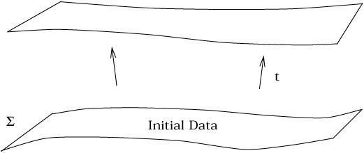
|
Since the metric is the fundamental variable, our first guess is that
we should consider the values
g![]()
![]() |
|![]() of the metric on our
hypersurface to be the "coordinates" and the time derivatives
of the metric on our
hypersurface to be the "coordinates" and the time derivatives
![]() g
g![]()
![]() |
|![]() (with respect to some specified time coordinate)
to be the "momenta", which together specify the state. (There
will also be coordinates and momenta for the matter fields, which we
will not consider explicitly.) In fact the equations
G
(with respect to some specified time coordinate)
to be the "momenta", which together specify the state. (There
will also be coordinates and momenta for the matter fields, which we
will not consider explicitly.) In fact the equations
G![]()
![]() = 8
= 8![]() GT
GT![]()
![]() do involve second derivatives of the
metric with respect to
time (since the connection involves first derivatives of the metric and
the Einstein tensor involves first derivatives of the connection),
so we seem to be on the right track. However, the Bianchi identity
tells us that
do involve second derivatives of the
metric with respect to
time (since the connection involves first derivatives of the metric and
the Einstein tensor involves first derivatives of the connection),
so we seem to be on the right track. However, the Bianchi identity
tells us that
![]() G
G![]()
![]() = 0. We can rewrite this equation as
= 0. We can rewrite this equation as
| (4.81) |
A close look at the right hand side reveals that there are no
third-order time derivatives; therefore there cannot be any
on the left hand side. Thus, although
G![]()
![]() as a whole involves
second-order time derivatives of the metric, the specific components
G0
as a whole involves
second-order time derivatives of the metric, the specific components
G0![]() do not. Of the ten independent
components in Einstein's
equations, the four represented by
do not. Of the ten independent
components in Einstein's
equations, the four represented by

| (4.82) |
cannot be used to evolve the initial data
(g![]()
![]() ,
,![]() g
g![]()
![]() )
)![]() .
Rather, they serve as constraints on this initial data; we are
not free to specify any combination of the metric and its time
derivatives on the hypersurface
.
Rather, they serve as constraints on this initial data; we are
not free to specify any combination of the metric and its time
derivatives on the hypersurface ![]() , since they must obey the
relations (4.82). The remaining equations,
, since they must obey the
relations (4.82). The remaining equations,

| (4.83) |
are the dynamical evolution equations for the metric. Of course,
these are only six equations for the ten unknown functions
g![]()
![]() (x
(x![]() ), so the solution will inevitably
involve a fourfold
ambiguity. This is simply the freedom that we have already mentioned,
to choose the four coordinate functions throughout spacetime.
), so the solution will inevitably
involve a fourfold
ambiguity. This is simply the freedom that we have already mentioned,
to choose the four coordinate functions throughout spacetime.
It is a straightforward but unenlightening exercise to sift through
(4.83) to find that not all second time derivatives of the metric
appear. In fact we find that
![]() gij appears in (4.83), but
not
gij appears in (4.83), but
not
![]() g0
g0![]() . Therefore a "state" in general relativity
will consist of a specification of the spacelike components of the
metric
gij|
. Therefore a "state" in general relativity
will consist of a specification of the spacelike components of the
metric
gij|![]() and their first time derivatives
and their first time derivatives
![]() gij|
gij|![]() on the hypersurface
on the hypersurface ![]() , from which we can
determine the future evolution using (4.83), up to an unavoidable
ambiguity in fixing the remaining components g0
, from which we can
determine the future evolution using (4.83), up to an unavoidable
ambiguity in fixing the remaining components g0![]() . The
situation is precisely analogous to that in electromagnetism, where
we know that no amount of initial data can suffice to determine the
evolution uniquely since there will always be the freedom to perform
a gauge transformation
A
. The
situation is precisely analogous to that in electromagnetism, where
we know that no amount of initial data can suffice to determine the
evolution uniquely since there will always be the freedom to perform
a gauge transformation
A![]()
![]() A
A![]() +
+ ![]()
![]() .
In general relativity, then, coordinate transformations play a role
reminiscent of gauge transformations in electromagnetism, in that
they introduce ambiguity into the time evolution.
.
In general relativity, then, coordinate transformations play a role
reminiscent of gauge transformations in electromagnetism, in that
they introduce ambiguity into the time evolution.
One way to cope with this problem is to simply "choose a gauge."
In electromagnetism this means to place a condition on the vector
potential A![]() , which will restrict our freedom to
perform gauge
transformations. For example we can choose Lorentz gauge, in which
, which will restrict our freedom to
perform gauge
transformations. For example we can choose Lorentz gauge, in which
![]() A
A![]() = 0, or temporal gauge, in which
A0 = 0. We can
do a similar thing in general relativity, by fixing our coordinate
system. A popular choice is harmonic gauge (also known as
Lorentz gauge and a host of other names), in which
= 0, or temporal gauge, in which
A0 = 0. We can
do a similar thing in general relativity, by fixing our coordinate
system. A popular choice is harmonic gauge (also known as
Lorentz gauge and a host of other names), in which

| (4.84) |
Here
![]() =
= ![]()
![]() is the covariant D'Alembertian,
and it is crucial to realize when we take the covariant derivative
that the four functions x
is the covariant D'Alembertian,
and it is crucial to realize when we take the covariant derivative
that the four functions x![]() are just functions, not components
of a vector. This condition is therefore simply
are just functions, not components
of a vector. This condition is therefore simply
| (4.85) |
In flat space, of course, Cartesian coordinates (in which
![]() = 0) are harmonic
coordinates. (As a
general principle, any function f which satisfies
= 0) are harmonic
coordinates. (As a
general principle, any function f which satisfies ![]() f = 0
is called an "harmonic function.")
f = 0
is called an "harmonic function.")
To see that this choice of coordinates successfully fixes our gauge freedom, let's rewrite the condition (4.84) in a somewhat simpler form. We have
| (4.86) |
from the definition of the Christoffel symbols. Meanwhile, from
![]() (g
(g![]()
![]() g
g![]()
![]() ) =
) = ![]()
![]() = 0 we have
= 0 we have
| (4.87) |
Also, from our previous exploration of the variation of the determinant of the metric (4.65), we have
| (4.88) |
Putting it all together, we find that (in general),
| (4.89) |
The harmonic gauge condition (4.85) therefore is equivalent to
| (4.90) |
Taking the partial derivative of this with respect to t = x0 yields
| (4.91) |
This condition represents a second-order differential equation
for the previously unconstrained metric components g0![]() , in
terms of the given initial data. We have therefore succeeded in
fixing our gauge freedom, in that we can now solve for the evolution
of the entire metric in harmonic coordinates. (At least locally;
we have been glossing over the fact our gauge choice may not be
well-defined globally, and we would have to resort to working in
patches as usual. The same problem appears in gauge theories in
particle physics.) Note that we still have some freedom remaining;
our gauge condition (4.84) restricts how the coordinates stretch from
our initial hypersurface
, in
terms of the given initial data. We have therefore succeeded in
fixing our gauge freedom, in that we can now solve for the evolution
of the entire metric in harmonic coordinates. (At least locally;
we have been glossing over the fact our gauge choice may not be
well-defined globally, and we would have to resort to working in
patches as usual. The same problem appears in gauge theories in
particle physics.) Note that we still have some freedom remaining;
our gauge condition (4.84) restricts how the coordinates stretch from
our initial hypersurface ![]() throughout spacetime, but we can
still choose coordinates xi on
throughout spacetime, but we can
still choose coordinates xi on ![]() however we like. This
corresponds to the fact that making a coordinate transformation
x
however we like. This
corresponds to the fact that making a coordinate transformation
x![]()
![]() x
x![]() +
+ ![]() , with
, with
![]()
![]() = 0,
does not violate the harmonic gauge condition.
= 0,
does not violate the harmonic gauge condition.
We therefore have a well-defined initial value problem for general
relativity; a state is specified by the spacelike components of the
metric and their time derivatives on a spacelike hypersurface ![]() ;
given these, the spacelike components (4.83) of Einstein's equations
allow us to evolve the metric forward in time, up to an ambiguity
in coordinate choice which may be resolved by choice of gauge.
We must keep in mind that the initial data are not arbitrary, but
must obey the constraints (4.82). (Once we impose the constraints on
some spacelike hypersurface, the equations of motion guarantee that they
remain satisfied, as you can check.) The constraints serve a useful
purpose, of guaranteeing that the result remains spacetime covariant
after we have split our manifold into "space" and "time."
Specifically, the
Gi0 = 8
;
given these, the spacelike components (4.83) of Einstein's equations
allow us to evolve the metric forward in time, up to an ambiguity
in coordinate choice which may be resolved by choice of gauge.
We must keep in mind that the initial data are not arbitrary, but
must obey the constraints (4.82). (Once we impose the constraints on
some spacelike hypersurface, the equations of motion guarantee that they
remain satisfied, as you can check.) The constraints serve a useful
purpose, of guaranteeing that the result remains spacetime covariant
after we have split our manifold into "space" and "time."
Specifically, the
Gi0 = 8![]() GTi0 constraint implies that
the evolution is independent of our choice of coordinates on
GTi0 constraint implies that
the evolution is independent of our choice of coordinates on
![]() , while
G00 = 8
, while
G00 = 8![]() GT00 enforces invariance under
different ways of slicing spacetime into spacelike hypersurfaces.
GT00 enforces invariance under
different ways of slicing spacetime into spacelike hypersurfaces.
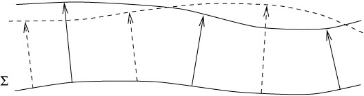
|
Once we have seen how to cast Einstein's equations as an initial value problem, one issue of crucial importance is the existence of solutions to the problem. That is, once we have specified a spacelike hypersurface with initial data, to what extent can we be guaranteed that a unique spacetime will be determined? Although one can do a great deal of hard work to answer this question with some precision, it is fairly simple to get a handle on the ways in which a well-defined solution can fail to exist, which we now consider.
It is simplest to first consider the problem of evolving matter fields
on a fixed background spacetime, rather than the evolution of the
metric itself. We therefore consider a spacelike hypersurface ![]() in some manifold M with fixed metric
g
in some manifold M with fixed metric
g![]()
![]() , and furthermore look
at some connected subset S in
, and furthermore look
at some connected subset S in ![]() . Our guiding principle will
be that no signals can travel faster than the speed of light; therefore
"information" will only flow along timelike or null trajectories
(not necessarily geodesics). We define the future domain of
dependence of S, denoted D+(S), as
the set of all points p such
that every past-moving, timelike or null, inextendible curve through
p must intersect S. ("Inextendible" just means that the curve
goes on forever, not ending at some finite point.) We interpret this
definition in such a way that S itself is a subset of
D+(S). (Of
course a rigorous formulation does not require additional interpretation
over and above the definitions, but we are not being as rigorous
as we could be right now.) Similarly, we
define the past domain of dependence D-(S) in
the same way, but
with "past-moving" replaced by "future-moving." Generally
speaking, some points in M will be in one of the domains of
dependence,
and some will be outside; we define the boundary of
D+(S) to be
the future Cauchy horizon H+(S), and
likewise the boundary of
D-(S) to be the past Cauchy horizon
H-(S). You can convince
yourself that they are both null surfaces.
. Our guiding principle will
be that no signals can travel faster than the speed of light; therefore
"information" will only flow along timelike or null trajectories
(not necessarily geodesics). We define the future domain of
dependence of S, denoted D+(S), as
the set of all points p such
that every past-moving, timelike or null, inextendible curve through
p must intersect S. ("Inextendible" just means that the curve
goes on forever, not ending at some finite point.) We interpret this
definition in such a way that S itself is a subset of
D+(S). (Of
course a rigorous formulation does not require additional interpretation
over and above the definitions, but we are not being as rigorous
as we could be right now.) Similarly, we
define the past domain of dependence D-(S) in
the same way, but
with "past-moving" replaced by "future-moving." Generally
speaking, some points in M will be in one of the domains of
dependence,
and some will be outside; we define the boundary of
D+(S) to be
the future Cauchy horizon H+(S), and
likewise the boundary of
D-(S) to be the past Cauchy horizon
H-(S). You can convince
yourself that they are both null surfaces.

|
The usefulness of these definitions should be apparent; if nothing
moves faster than light, than signals cannot propagate outside the
light cone of any point p. Therefore, if every curve which
remains inside this light cone must intersect S, then information
specified on S should be sufficient to predict what the situation
is at p. (That is, initial data for matter fields given on S
can be used to solve for the value of the fields at p.) The set
of all points for which we can predict what happens by knowing
what happens on S is simply the union
D+(S) ![]() D-(S).
D-(S).
We can easily extend these ideas from the subset S to the entire
hypersurface ![]() . The important point is that
D+(
. The important point is that
D+(![]() )
) ![]() D-(
D-(![]() ) might fail to be all of M, even if
) might fail to be all of M, even if ![]() itself
seems like a perfectly respectable hypersurface that extends
throughout space. There are a number of ways in which this can
happen. One possibility is that we have just chosen a "bad"
hypersurface (although it is hard to give a general prescription for
when a hypersurface is bad in this sense). Consider Minkowski space,
and a spacelike hypersurface
itself
seems like a perfectly respectable hypersurface that extends
throughout space. There are a number of ways in which this can
happen. One possibility is that we have just chosen a "bad"
hypersurface (although it is hard to give a general prescription for
when a hypersurface is bad in this sense). Consider Minkowski space,
and a spacelike hypersurface ![]() which remains to the past of
the light cone of some point.
which remains to the past of
the light cone of some point.

|
In this case ![]() is a nice spacelike surface, but
it is clear that
D+(
is a nice spacelike surface, but
it is clear that
D+(![]() ) ends at the light cone, and we cannot
use information on
) ends at the light cone, and we cannot
use information on ![]() to predict what happens throughout
Minkowski space. Of course, there are other surfaces we could have
picked for which the domain of dependence would have been the entire
manifold, so this doesn't worry us too much.
to predict what happens throughout
Minkowski space. Of course, there are other surfaces we could have
picked for which the domain of dependence would have been the entire
manifold, so this doesn't worry us too much.
A somewhat more nontrivial example is known as Misner space.
This is a two-dimensional spacetime with the topology of
![]() × S1, and a metric for
which the light cones progressively tilt as you go forward in time.
× S1, and a metric for
which the light cones progressively tilt as you go forward in time.

|
Past a certain point, it is possible to travel on a timelike
trajectory which wraps around the S1 and comes back to
itself; this
is known as a closed timelike curve. If we had specified a
surface ![]() to this past of this point, then none of the points
in the region containing closed timelike curves are in the domain of
dependence of
to this past of this point, then none of the points
in the region containing closed timelike curves are in the domain of
dependence of ![]() , since the closed timelike curves themselves
do not intersect
, since the closed timelike curves themselves
do not intersect ![]() . This is obviously a worse problem than
the previous one, since a well-defined initial value problem does not
seem to exist in this spacetime. (Actually problems like this are
the subject of some current research interest, so I won't claim that
the issue is settled.)
. This is obviously a worse problem than
the previous one, since a well-defined initial value problem does not
seem to exist in this spacetime. (Actually problems like this are
the subject of some current research interest, so I won't claim that
the issue is settled.)
A final example is provided by the existence of singularities, points which are not in the manifold even though they can be reached by travelling along a geodesic for a finite distance. Typically these occur when the curvature becomes infinite at some point; if this happens, the point can no longer be said to be part of the spacetime. Such an occurrence can lead to the emergence of a Cauchy horizon - a point p which is in the future of a singularity cannot be in the domain of dependence of a hypersurface to the past of the singularity, because there will be curves from p which simply end at the singularity.
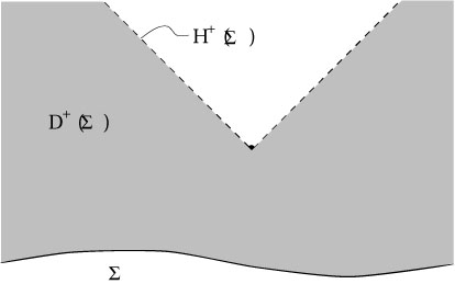
|
All of these obstacles can also arise in the initial value problem for GR, when we try to evolve the metric itself from initial data. However, they are of different degrees of troublesomeness. The possibility of picking a "bad" initial hypersurface does not arise very often, especially since most solutions are found globally (by solving Einstein's equations throughout spacetime). The one situation in which you have to be careful is in numerical solution of Einstein's equations, where a bad choice of hypersurface can lead to numerical difficulties even if in principle a complete solution exists. Closed timelike curves seem to be something that GR works hard to avoid - there are certainly solutions which contain them, but evolution from generic initial data does not usually produce them. Singularities, on the other hand, are practically unavoidable. The simple fact that the gravitational force is always attractive tends to pull matter together, increasing the curvature, and generally leading to some sort of singularity. This is something which we apparently must learn to live with, although there is some hope that a well-defined theory of quantum gravity will eliminate the singularities of classical GR.