


7.4 Nonlinear Fits
As we have already mentioned, nonlinear fits generally require a numerical procedure for minimizing S. Function minimization or maximization (2) is a problem in itself and a number of methods have been developed for this purpose. However, no one method can be said to be applicable to all functions, and, indeed, the problem often is to find the right method for the function or functions in question. A discussion of the different methods available, of course, is largely outside the scope of this book. However, it is nevertheless worthwhile to briefly survey the most used methods so as to provide the reader with a basis for more detailed study and an idea of some of the problems to be expected. For practical purposes, a computer is necessary and we strongly advise the reader to find a ready-made program rather than attempt to write it himself. More detailed discussions may be found in [Refs: 9, 10, 11].
Function Minimization Techniques. Numerical minimization methods are generally iterative in nature, i.e., repeated calculations are made while varying the parameters in some way, until the desired minimum is reached. The criteria for selecting a method, therefore, are speed and stability against divergences. In general, the methods can be classified into two broad categories: grid searches and gradient methods.
The grid methods are the simplest. The most elementary procedure is
to form a grid of equally spaced points in the variables of interest
and evaluate the function at each of these points. The point with the
smallest value is then the approximate minimum. Thus, if F(x) is the
function to minimize, we would evaluate F at
x0,
x0 +  x, x0 +
2x,
etc. and choose the point x' for which F is smallest. The
size of the
grid step, x, depends on
the accuracy desired. This method, of
course, can only be used over a finite range of x and in cases
where x
ranges over infinity it is necessary to have an approximate idea of
where the minimum is. Several ranges may also be tried.
x, x0 +
2x,
etc. and choose the point x' for which F is smallest. The
size of the
grid step, x, depends on
the accuracy desired. This method, of
course, can only be used over a finite range of x and in cases
where x
ranges over infinity it is necessary to have an approximate idea of
where the minimum is. Several ranges may also be tried.
The elementary grid method is intrinsically stable, but it is quite obviously inefficient and time consuming. Indeed, in more than one dimension, the number of function evaluations becomes prohibitively large even for a computer! (In contrast to the simple grid method is the Monte Carlo or random search. Instead of equally spaced points, random points are generated according to some distribution, e.g., a uniform density.)
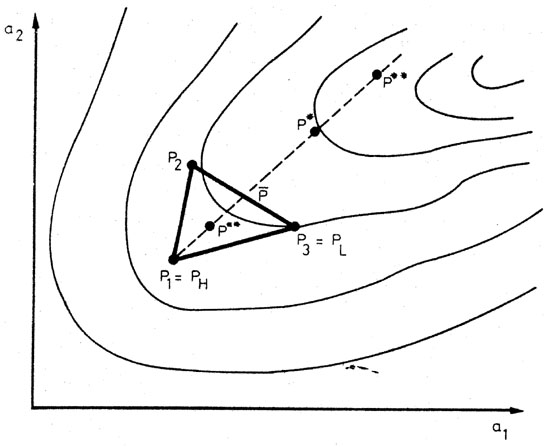
More efficient grid searches make use of variable stepping methods so as to reduce the number of evaluations while converging onto the minimum more rapidly. A relatively recent technique is the simplex method [Ref. 12]. A simplex is the simplest geometrical figure in n dimensions having n + 1 vertices. In n = 2 dimensions, for example, the simplex is a triangle while in n = 3 dimensions, the simplex is a tetrahedron, etc. The method takes on the name simplex because it uses n + 1 points at each step. As an illustration, consider a function in two dimensions, the contours of which are shown in Fig. 8. The method begins by choosing n + 1 = 3 points in some way or another, perhaps at random. A simplex is thus formed as shown in the figure. The point with the highest value is denoted as PH, while the lowest is PL. The next step is to replace PH with a better point. To do this, PH is reflected through the center of gravity of all points except PH, i.e., the point
This yields the point P* =
 +
( -
PH). If F(P*) <
F(PL), a new
minimum has been found and an attempt is made to do even better by
trying the point P** =
2( -
PH). The best point is then kept. If
F(P*) > F(PH) the
reflection is brought backwards to P** =
- 1/2
( -
PH). If this is not better than PH,
a new simplex is formed with
points at Pi = (Pi +
PL) / 2 and the procedure restarted. In this
manner, one can imagine the triangle in
Fig. 8 ``falling'' to the
minimum. The simplex technique is a good method since it is relatively
insensitive to the type of function, but it can also be rather slow.
+
( -
PH). If F(P*) <
F(PL), a new
minimum has been found and an attempt is made to do even better by
trying the point P** =
2( -
PH). The best point is then kept. If
F(P*) > F(PH) the
reflection is brought backwards to P** =
- 1/2
( -
PH). If this is not better than PH,
a new simplex is formed with
points at Pi = (Pi +
PL) / 2 and the procedure restarted. In this
manner, one can imagine the triangle in
Fig. 8 ``falling'' to the
minimum. The simplex technique is a good method since it is relatively
insensitive to the type of function, but it can also be rather slow.
|
Fig. 8. The simplex method for function minimization. |
Gradient methods are techniques which make use of the derivatives of the function to be minimized. These can either be calculated numerically or supplied by the user if known. One obvious use of the derivatives is to serve as guides pointing in the direction of decreasing F. This idea is used in techniques such as the method of steepest descent. A more widely used technique, however, is Newton's method which uses the derivatives to form a second-degree Taylor expansion of the function about the point x0,
In n dimensions, this is generalized to
 F(x0) + gT
(x - x0) + 1/2 (x
- x0)T
F(x0) + gT
(x - x0) + 1/2 (x
- x0)T
 (x -
x0)
(x -
x0)
where gi is the vector of first derivatives ðF / ðxi and Gij the matrix of second derivatives ð2F / ðxi ðxj. The matrix G is also called the Hessian. In essence, the method approximates the function around x0 by a quadratic surface. Under this assumption, it is very easy to calculate the minimum of the n dimensional parabola analytically,
-1
g .
This, of course, is not the true minimum of the function; but by
forming a new parabolic surface about xmin and
calculating its
minimum, etc., a convergence to the true minimum can be obtained
rather rapidly. The basic problem with the technique is that it
requires to
be everywhere positive definite, otherwise at some point
in the iteration a maximum may be calculated rather than a minimum,
and the whole process diverges. This is more easily seen in the
one-dimensional case in (86). If the second derivative is negative,
then, we clearly have an inverted parabola rather than the desired
well-shape figure.
Despite this defect, Newton's method is quite powerful and
algorithms have been developed in which the matrix
is artificially
altered whenever it becomes negative. In this manner, the iteration
continues in the right direction until a region of
positive-definiteness is reached. Such variations are called
quasi-Newton methods.
The disadvantage of the Newton methods is that each iteration
requires an evaluation of the matrix
and its
inverse. This, of
course, becomes quite costly in terms of time. This problem has given
rise to another class of methods which either avoid calculating G or
calculate it once and then ``update'' G with some correcting function
after each iteration. These methods are described in more detail by
James
[Ref. 11].
In the specific case of least squares minimization, a common procedure used with Newton's method is to linearize the fitting function. This is equivalent to approximating the Hessian in the following manner. Rewriting (70) as

where sk = [yk -
f(xk)] /  k, the Hessian becomes
The second term in the sum can be considered as a second order correction and is set to zero. The Hessian is then
This approximation has the advantage of ensuring positive-definiteness and the result converges to the correct minimum. However, the covariance matrix will not in general converge to the correct covariance values, so that the errors as determined by this matrix may not be correct.
As the reader can see, it is not a trivial task to implement a nonlinear least squares program. For this reason we have advised the use of a ready-made program. A variety of routines may be found in the NAG library [Ref. 13], for example. A very powerful program allowing the use of a variety of minimization methods such a simplex, Newton, etc., is Minuit [Ref. 14] which is available in the CERN program library. This library is distributed to many laboratories and universities.
Local vs Global Minima. Up to now we have assumed that the function F contains only one minimum. More generally, of course, an arbitrary function can have many local minima in addition to a global, absolute minimum. The methods we have described are all designed to locate a local minimum without regard for any other possible minima. It is up to the user to decide if the minimum obtained is indeed what he wants. It is important, therefore, to have some idea of what the true values are so as to start the search in the right region. Even in this case, however, there is no guarantee that the process will converge onto the closest minimum. A good technique is to fix those parameters which are approximately known and vary the rest. The result can then be used to start a second search in which all the parameters are varied. Other problems which can arise are the occurrence of overflow or underflow in the computer. This occurs very often with exponential functions. Here good starting values are generally necessary to obtain a result.
Errors. While the methods we have discussed allow us to find the
parameter values which minimize the function S, there is no
prescription for calculating the errors on the parameters. A clue,
however, can be taken from the linear one-dimensional case. Here we
saw the variance of a parameter
 was given by the inverse of the
second derivative (92),
was given by the inverse of the
second derivative (92),
If we expand S in Taylor series about the minimum
At the point =
* +
, we thus find that
Thus the error on corresponds
to the distance between the minimum and
where the S distribution increases by 1.
This can be generalized to the nonlinear case where the S distribution is not generally parabolic around the minimum. Finding the errors for each parameter then implies finding those points for which the S value changes by 1 from the minimum. If S has a complicated form, of course, this is not always easy to determine and once again, a numerical method must be used to solve the equation. If the form of S can be approximated by a quadratic surface, then, the error matrix in (73) can be calculated and inverted as in the linear case. This should then give an estimate of the errors and covariances.
2 A minimization can be turned into a maximization by simply adding a minus sign in front of the function and vice-versa. Back.